Difference between revisions of "Training Material for UN Open GIS OpenData"
| Line 62: | Line 62: | ||
Then, we will cut all layers by the boundary of the selected county, Tabora. <br/> | Then, we will cut all layers by the boundary of the selected county, Tabora. <br/> | ||
Firstly, export from the administrative units level 1, Tabora county. Secondly, clip all layers by its geometry. | Firstly, export from the administrative units level 1, Tabora county. Secondly, clip all layers by its geometry. | ||
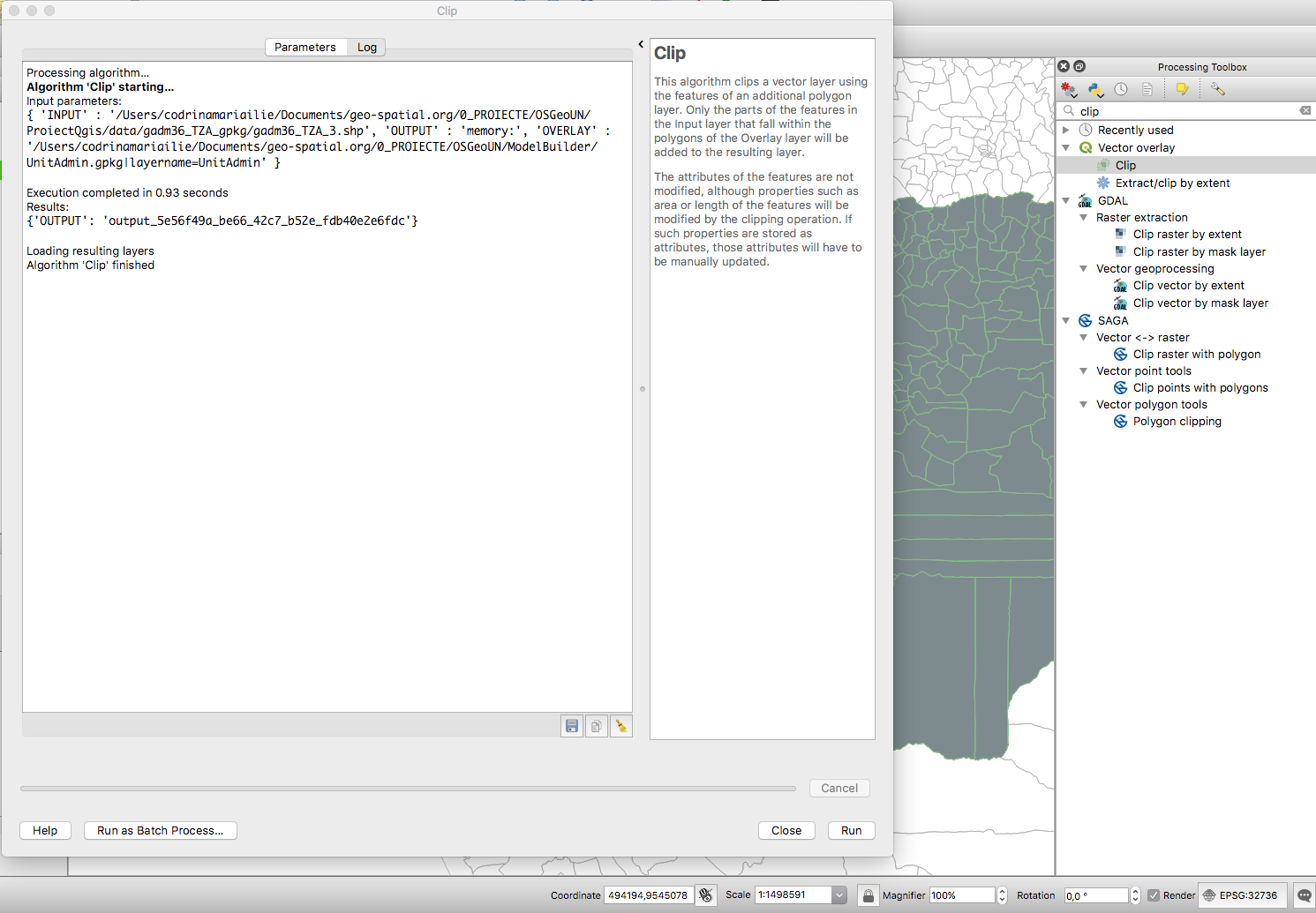
| − | [[File:fig2_clip.png|thumb|center|800px| Clip tool identified in the Processing toolbox]] | + | [[File:fig2_clip.png|thumb|center|800px|Fig. 2 Clip tool identified in the Processing toolbox]] |
====Step 3==== | ====Step 3==== | ||
| Line 71: | Line 71: | ||
Step 4 prepares the dataset from which we will extract the population number for all rural areas of each administrative unit. We will use zonal statistics, a tool now available in the Processing Toolbox. | Step 4 prepares the dataset from which we will extract the population number for all rural areas of each administrative unit. We will use zonal statistics, a tool now available in the Processing Toolbox. | ||
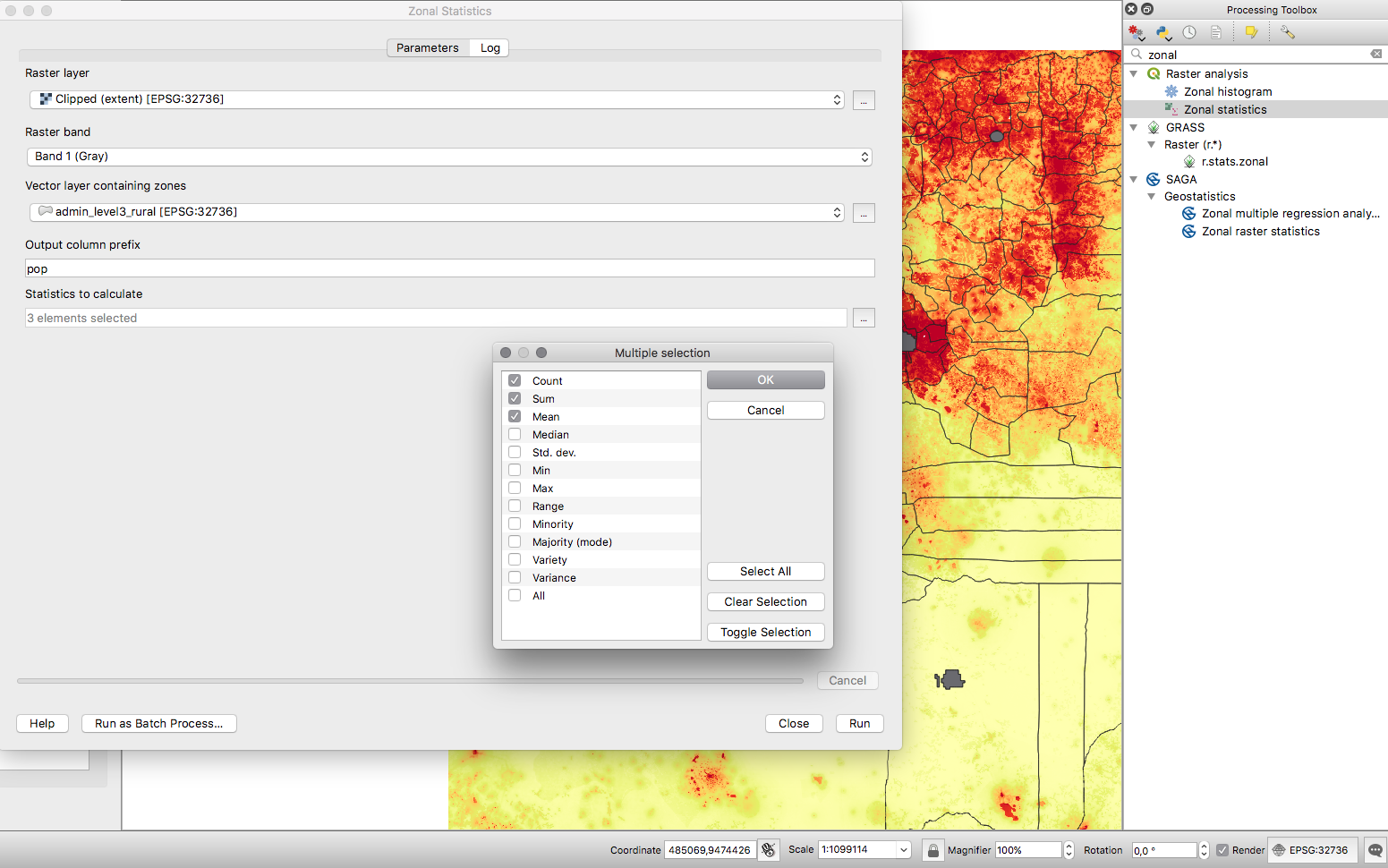
| − | [[File:fig4_zonalStats.png|thumb|center|800px|Zonal statistics ran on the administrative units - rural extent]] | + | [[File:fig4_zonalStats.png|thumb|center|800px|Fig.3 Zonal statistics ran on the administrative units - rural extent]] |
====Step 5==== | ====Step 5==== | ||
| Line 112: | Line 112: | ||
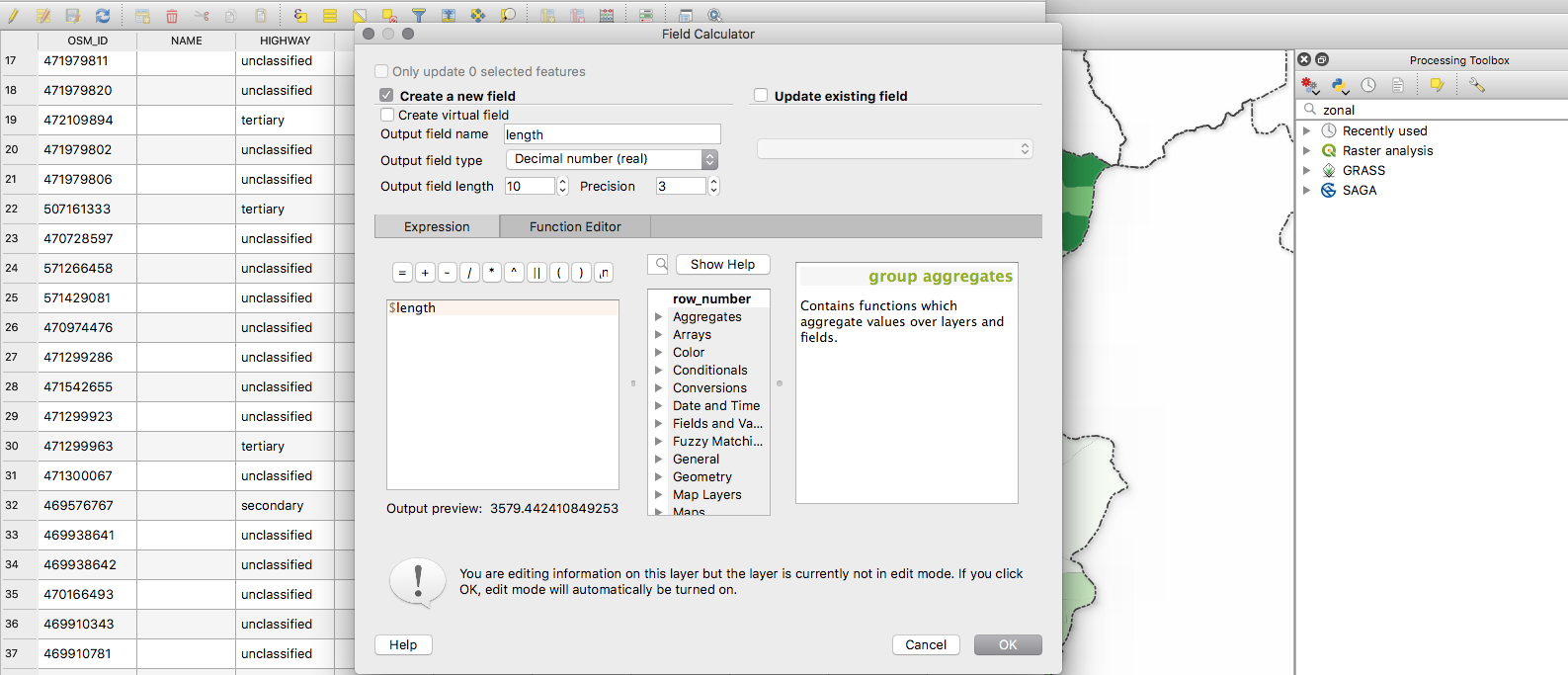
To calculate the roads length, we open the attribute table of the dataset, we create a new column and we write $length. | To calculate the roads length, we open the attribute table of the dataset, we create a new column and we write $length. | ||
| − | [[File:fig5_length.png|thumb|center|800px|Calculating the roads length]] | + | [[File:fig5_length.png|thumb|center|800px|Fig. 4 Calculating the roads length]] |
The next step leading to the RAI calculation is to determine the road condition that will be taken into account. This represents a difficult assessment to make, mainly due to lack of harmonization between OpenStreetMap defined tags and official internationally used methodologies for road condition calculations. For the purpose of our exercise, we will consider the proposed definition of what a “road in good condition” given in the World Bank 2016 document Measuring Rural Access: Using New Technologies (Transport & ICT. WB, 2016.): <br/> | The next step leading to the RAI calculation is to determine the road condition that will be taken into account. This represents a difficult assessment to make, mainly due to lack of harmonization between OpenStreetMap defined tags and official internationally used methodologies for road condition calculations. For the purpose of our exercise, we will consider the proposed definition of what a “road in good condition” given in the World Bank 2016 document Measuring Rural Access: Using New Technologies (Transport & ICT. WB, 2016.): <br/> | ||
| Line 143: | Line 143: | ||
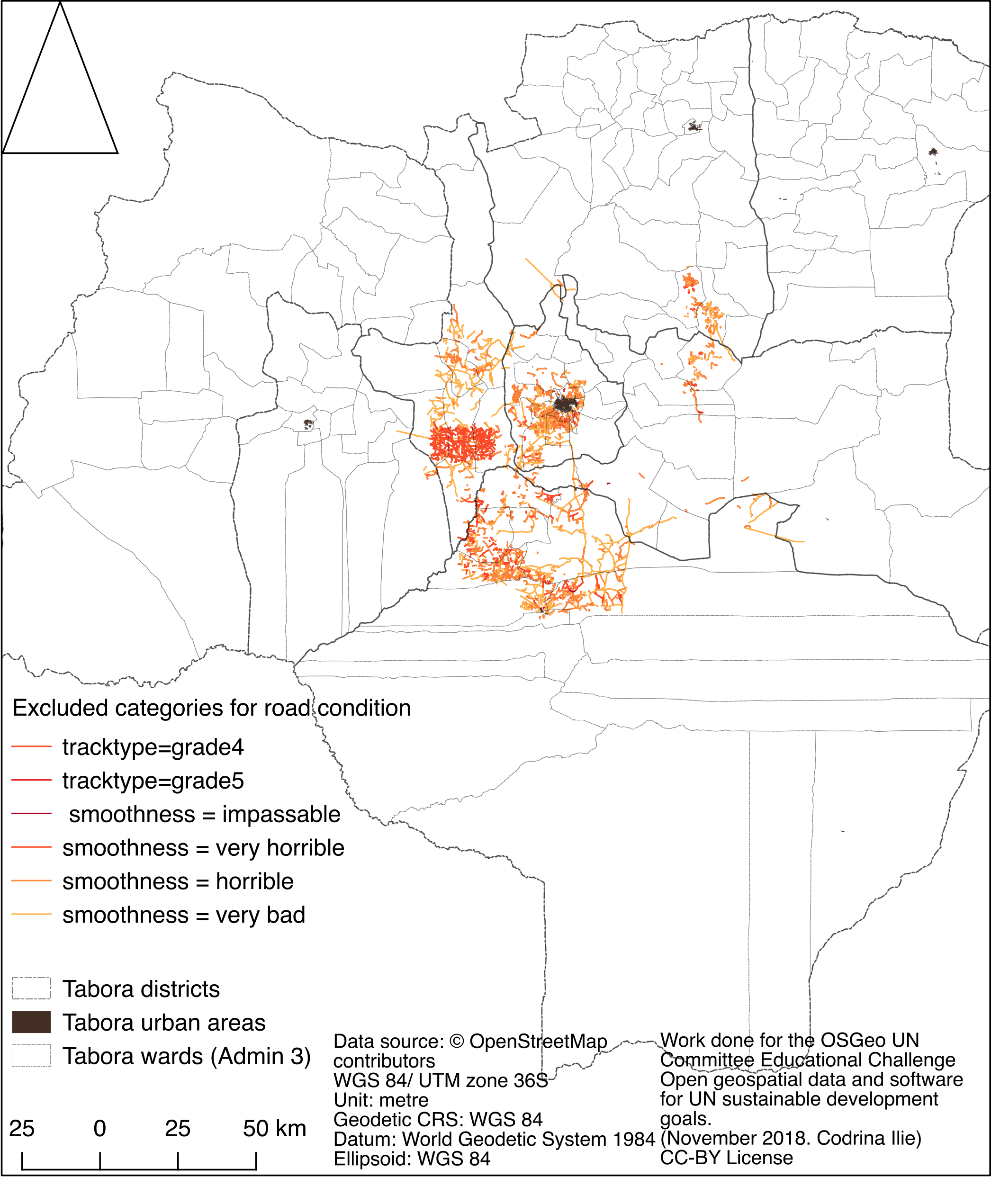
The spatial distribution of the roads eliminated from our analysis is presented in the map below: | The spatial distribution of the roads eliminated from our analysis is presented in the map below: | ||
| − | [[File:fig10_excludedRoads.png|thumb|center|500px|Spatial distribution of the excluded road condition categories]] | + | [[File:fig10_excludedRoads.png|thumb|center|500px|Fig. 6 Spatial distribution of the excluded road condition categories]] |
After a quick glance, we can see that a significant central rural area is served by the roads with a too poor condition to be included in the RAI calculation. | After a quick glance, we can see that a significant central rural area is served by the roads with a too poor condition to be included in the RAI calculation. | ||
Revision as of 03:36, 21 January 2019
Introduction
Scope
The following educational material has been drafted within the framework of the OSGeo UN Committee Educational Challenge - Open Geospatial Data and software for UN sustainable development goals. The overarching goal is to show that at this time, the combination of open (geo)data globally available and the significant developments of the free and open source solutions for geospatial is sufficient to initiate geospatial analysis, at worldwide level, at small and intermediate scales, to better understand our ecosystem. In that respect, we have employed OSGeo software solutions to process global open geospatial datasets to answer one selected indicator for a sustainable development goal. The selected indicator is 9.1.1 Proportion of the rural population who live within 2 km of an all-season road (C0901010) which supports the target of developing quality, reliable, sustainable and resilient infrastructure, including regional and transborder infrastructure, to support economic development and human well-being, with a focus on affordable and equitable access for all. The indicator has been chosen after a close analysis of all SGDs and the corresponding indicators as to comply with the following:
- to have a spatial dimension;
- to not be an indicator that is already addressed through another initiative, such as the GEO Wetlands Initiative, WHO Interactive Air Pollution Maps, GEO AquaWatch, ESA CoastColour etc.;
- if possible, to not be yet the subject of a published methodology.
Audience
We have prepared this educational material for researchers, educators and professionals in local, regional, national or international agencies with minimal to intermediate geospatial information knowledge. We assume our audience has already basic knowledge of geospatial data structures, formats and that they have already used a GIS software, as to have basic skills and understanding of how to work with geospatial and tabular data. In that respect, we have limited the interactions with the command line, however we have inserted references to it.
Data and software used
Datasets and software used For the calculation of the SDG indicator, we have only used QGIS 3.4. We have also taken into consideration that changes that might occur from one version to another and thus focused on the functions used more than on a step-by-step guide. The datasets used for our exercise are the following:
Acquired knowledge
After going through the entire educational material, one will be able to:
- Have a broader view on what are the types of geospatial data open at global scale, as well as what are their limitations.
- Have a more deeper understanding of working with geospatial data using a dedicated software
- Consistent knowledge of QGIS software fundamentals
- Learn how to create cartographic representations of the obtained results
Educational Material
Open geospatial information and its role in answering UN Sustainable Development Goals
Population dataset description
Global Administrative Units Dataset description
For road related data, we have decided to use OpenStreetMap data as it is the only homogeneously designed globally available dataset. Without doubt, the amount and the quality of the available data for various regions around the world can vary consistently. However, given the clear and consistent definition of each map element and tag, this exercise should be reproducible in any other part of the world.
Yet, given our area of interest, the Tabora county from Tanzania, we must take into consideration specific developments for Africa, more precisely, the Highway Tag Africa - Topology of Road Network in African countries, and furthermore, the East Africa Tagging Guidelines.
However, with consideration to the global replicability of our educational material, we will also insert specifications on a more general scale. Of course, it must be acknowledged that the workflow presented here could require other adjustments with respect to the specificity of the road dataset used in calculation.
Preparing the geospatial data
For the scope of this exercise we have chosen the Tabora county of Tanzania. As we strive to create an educational material that can be applied no matter the region of interest, a decision was made to use the available datasets, on a global level.
The following table presents the datasets used:
| Topic | Name collection/dataset | Abstract | Indicators | Produce/collector | Owner | License | Type of data | Format | Scale/spatial resolution | Edition | CRS | Other URL |
|---|---|---|---|---|---|---|---|---|---|---|---|---|
| Administrative units | Database of Global Administrative Areas | GADM provides maps and spatial data for all countries and their sub-divisions. | administrative units | University of California, Berkeley,Museum of Vertebrate Zoology, and theInternational Rice Research Institute (Global Administrative Areas 2009) | GDAM | The data are freely available for academic use and other non-commercial use. Redistribution, or commercial use is not allowed without prior permission. | vector | Geopackage, shapefile, geodatabase. KMZ, R formats | n/a | April 2018 | Geographic WGS84 | https://gadm.org/metadata.html |
| World Population | WorldPop | Alpha version 2010 and 2015 estimates of numbers of people per grid square, with national totals adjusted to match UN population division estimates (http://esa.un.org/wpp/) and remaining unadjusted. | Settelments, Population numbers, birth and pregnancy, age structures, poverty spatial distribution etc. | GeoData Institute, University of Southampton | GeoData Institute, University of Southampton | CC BY 4.0 | raster | GeoTIFF | 100 m | July 2013 | Geographic WGS84 | http://www.worldpop.org.uk/data/methods/ |
| World Population | Global Rural-Urban Mapping project (GRUMP), v1 | To provide a polygon representation of urban areas with city or agglomeration name and time series population estimates. | urban geometries | Socioeconomic Data and Applications Center (sedac) | Socioeconomic Data and Applications Center (sedac) | CC BY 4.0 | vector | shapefile | 30 arc-second | 2006 | Geographic WGS84 | n/a |
| World Population | Global Human Built-up And Settlement Extent (HBASE) Dataset From Landsat, v1 (2010) | To provide high spatial resolution estimates of global urban extent derived from global 30m Landsat satellite data for the target year 2010 and a companion dataset to the Global Man-made Impervious Surface (GMIS) dataset. | urban extent | Socioeconomic Data and Applications Center (sedac) | Socioeconomic Data and Applications Center (sedac) | CC BY 4.0 | raster | GeoTiff | 30 m | 2017 | Geographic WGS84, UTM | n/a |
| OpenStreetMap | OpenStreetMap) | OpenStreetMap is built by a community of mappers that contribute and maintain data about roads, trails, cafés, railway stations, and much more, all over the world. | road network, road condition | OpenStreetMap contributors | OpenStreetMap Foundation (OSMF) | Open Data Commons Open Database License (ODbL) | vector | osm | n/a | September 2018 | Pseudo-Mercator, EPSG 3857 | https://wiki.openstreetmap.org/wiki/Main_Page |
Step 1
Add all listed data to your project. Create group layers as you bring in the data, so it is easier when you start processing to navigate through all datasets. Create and save your project, so you can pick up the work from where you left it.
/
[Layer]-->[Add layer] - will open the Data Source Manager that allows you to load the data.: the administrative unites (GDAM dataset), the population numbers (WorldPop - we will use the TZA_popmap15adj_v2b.tif file), the urban extent (we will use the global_urban_extent_polygons_v1.01.shp file).
As mentioned, we will use OpenStreetMap data for the roads geometry and condition. Bringing OSM data will require you install a new plugin - OSM Downloader.
[Plugins]-->[Manage and install plugins].
Step 2
The datasets are in various projections, either the Geographic projection EPSG 4326 or the Pseudo_Mercator EPSG 3857. A geographic coordinate system is based on a spheroid and uses angular units (degrees). Thus, when using QGIS calculator, for example, it returns values in decimal degree and not meters. You can see the used units in a projection's description that can be retrieved from epsg.io. [1]
As we will work with road geometries, we must reproject all the datasets in a projected coordinate system, which is based on a 2D plane (with the spheroid projected on a 2D plane) and uses linear units, such as meters. For our study, we identify a suitable CRS [2] for our region of interest, the Tabora county in Tanzania. To do that we will use epsg.io. After a quick search, we find WGS 84 / UTM zone 36S-EPSG: 32736 to be the appropriate for our region.
To reproject vector data using QGIS, we have to save the file with the desired projection.
Click on the vector layer you want to reproject and choose [Export]-->[Save features as..]
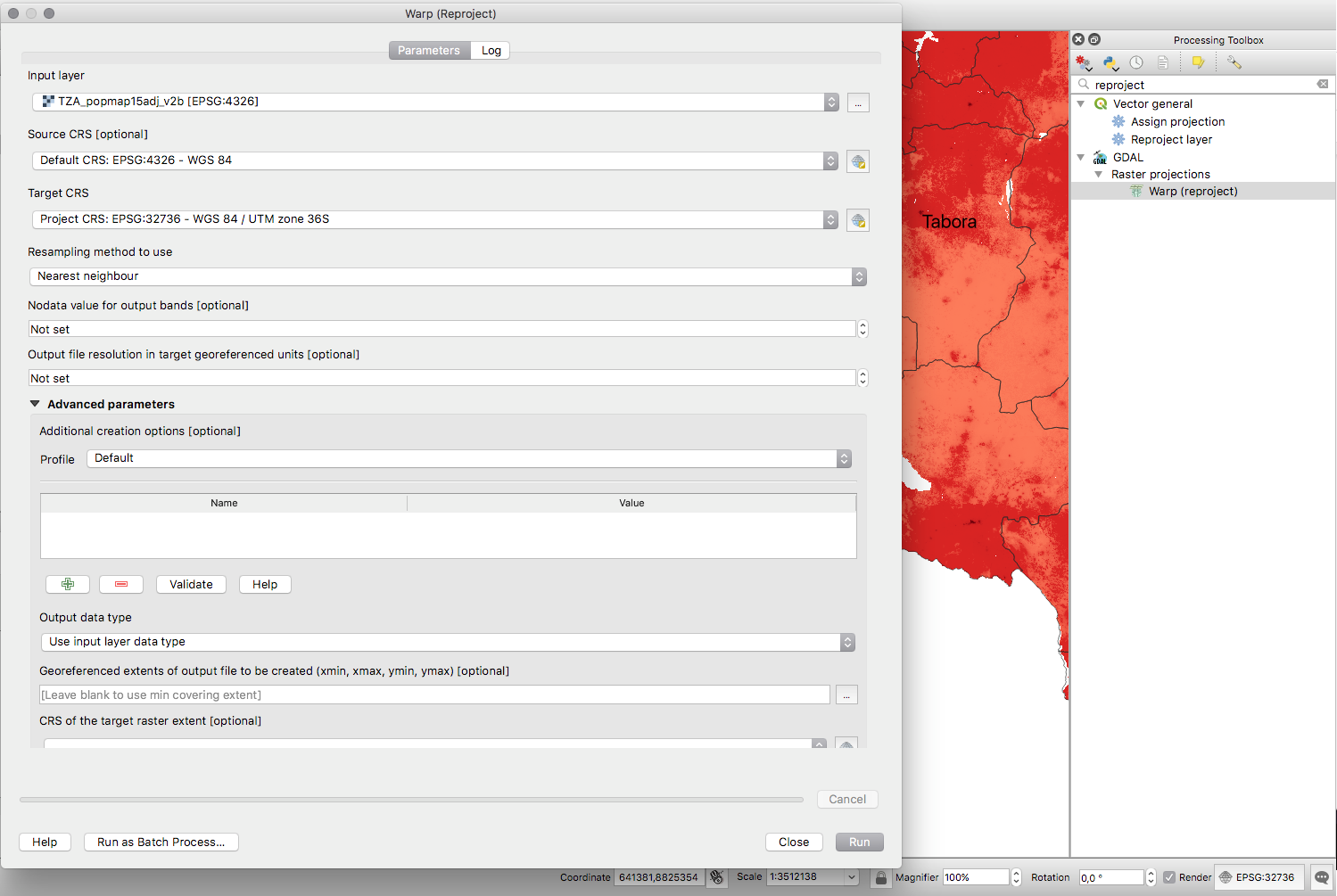
For raster datasets, we will use gdalwrap that is available as a processing tool in the Processing toolbox.
[Processing]-->[Toolbox]
We can search by typing the keyword 'reproject' in the search bar.
Then, we will cut all layers by the boundary of the selected county, Tabora.
Firstly, export from the administrative units level 1, Tabora county. Secondly, clip all layers by its geometry.
Step 3
Step 3 produces the rural areas of the Tabora county. According to Wikipedia, Tanzania is divided into regions (GDAM administrative level 1), districts (GDAM administrative level 2) and wards, (GDAM administrative level 3).
We will calculate the Rural Access Index on wards, thus we will extract the rural regions from the administrative units level 3. The resulting dataset will be vector type.
[Vector]-->[Geoprocessing tools]-->[Difference]
Step 4
Step 4 prepares the dataset from which we will extract the population number for all rural areas of each administrative unit. We will use zonal statistics, a tool now available in the Processing Toolbox.
Step 5
Bring in the roads!
Step 5 is the most time consuming processing stage and, more over, it may vary when this exercise will be applied to other regions in the world. For the roads geometry and condition we will use the OpenStreetMap data available.
As we will see, Tanzania is very well represented on the OSM map, even if we will encounter various situations mainly regarding quality of network connectivity, an important aspect for our study. That is because in 2015, the Crowd2Map Tanzania was launched and during the following years, there have been significant crowd mapping campaigns.
After step 1 and 2, the road dataset should be imported into QGIS, clipped, reprojected in EPSG 32736 and saved as a geopackage file.
Next, we will do a preliminary cleaning, by eliminating all roads segments that are not suitable for cars. The SDG indicator 9.1.1 Proportion of the rural population who live within 2 km of an all-season road refers to roads that are suitable for any kind of vehicle (average modern automobile), thus we will filtrate by:
"highway" = 'cycleway' or "highway" = 'pedestrian' or "highway" = 'path' or "highway" = 'footway' or "highway" = ‘residential’ or "highway" = ‘service’. We have also deleted roads under construction, because that means that the roads can not be used for access.
OpenStreetMap defines map features by tags. Each tag has 2 elements: the key and the value. The key is used to describe a topic, category, or type of feature and the value describes the specific form of the key-specified feature. In our filter above, the tag "highway" = 'cycleway' is formed by the key "highway" and the value 'cycleway', which means that the map feature is a road for bicycles. More details on how OpenStreetMap is build can be found in the OSM wiki.
There is a number of tags considered in OSM road data that gives important indication related to the road condition. These are:
- Key:smoothness with 8 possible values: excellent, good, intermediate, bad, very_bad, horrible, very_horrible, impassable. According to the OSM community, in developing countries, the HDM model is using some values of smoothness to help define road quality. The HDM stands for Highway Development and Management (HDM-4) and it represents the World Bank tool for the management of roads network, particularly in developing countries.
- Key: surface
- Key:surface:grade
- Tag: tracktype with a gradual variation from grade1 - solid to grade5 - soft.
Considering the East Africa Tagging Guidelines, there is an emphasis in using surface=* with the generic separation of surface=paved for sealed roads and surface=unpaved for the others. Analyzing the available data for the area of interest, the Tabora county of Tanzania, we can identify that for a number of road segments, we have road quality particular tags identified. We can see that in the other_tags column. Looking at the structure of the attributes registered in this column, we observe a number of things:
- The tags (key+value) are separated by comma;
- The keys are separated by their values through "=>" ;
- Tags are not necessarily in the same order;
- Not all tags that are relevant for our exercise are registered.
To simplify the processing steps, we will break the other_tags column into one column per tag. We will do this using an external solution, LibreOffice. The file containing the attributes for each segment is the .dbf file (dBase file) which can be opened and manipulated by tabular data solutions as well. It is advisable though that any change on the file to be done with caution, as it can corrupt the file, and thus make it unusable.
-->open .dbf file using LibreOffice --> Text to column by separator comma
Next, we create one column for each road condition key available: surface, smoothness and tracktype with the values specific for each road segment. Afterwards, we populate the three new columns (surface, smoothness and tracktype) with the specific value for each road segment. For this, we will use the Field Calculator of QGIS introducing the following expression:
 CASE
  WHEN  "other_tags" LIKE '%surface%'
  THEN  regexp_replace ("other_tags", 'surface"=>"', )
  ELSE surface
 END
where,
Other_tags - column from where we take the attribute value, and will be subsequently replaced by columns Tag1, Tag2 and so on for each of the three columns.
Surface - is the key name we are looking for in the attribute list.
After we have populated the three new columns (surface, smoothness and tracktype), we can extract information that will allow us to better understand the roads dataset we will use to calculate the RAI. We will make use of the statistics functionality of QGIS to show the total length of roads in our area of interest, but also various lengths, as for example the lengths of paved roads, or bad roads lengths and so on.
To calculate the roads length, we open the attribute table of the dataset, we create a new column and we write $length.
The next step leading to the RAI calculation is to determine the road condition that will be taken into account. This represents a difficult assessment to make, mainly due to lack of harmonization between OpenStreetMap defined tags and official internationally used methodologies for road condition calculations. For the purpose of our exercise, we will consider the proposed definition of what a “road in good condition” given in the World Bank 2016 document Measuring Rural Access: Using New Technologies (Transport & ICT. WB, 2016.):
"A road in good condition refers to:
* Paved road with IRI less than 6 meters/km and unpaved road with IRI less than 13 meters/km, when IRI data are available
* Paved road in excellent, good, or fair condition and unpaved road in excellent or good condition, when IRI data are not available but other road condition data, such as the PCI or visual assessment by class value, are available.
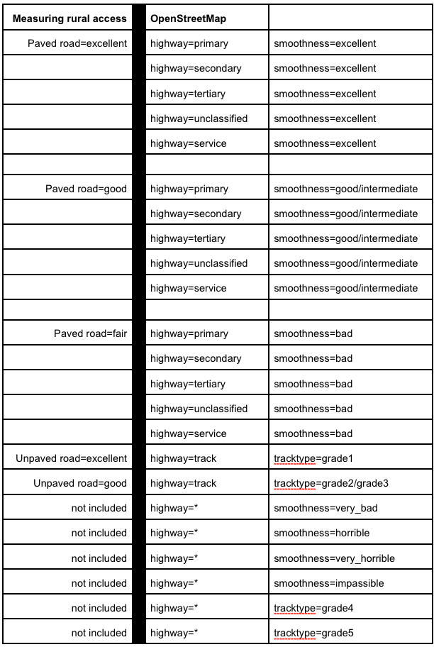
In our case, there is no available IRI data available, thus our data falls in the second category, where we have a qualitative description: Paved road in excellent, good, or fair condition and unpaved road in excellent or good condition. In order to work with available OSM road data, we will chart a compatibility map between OSM tags that describe road condition and the given classification.
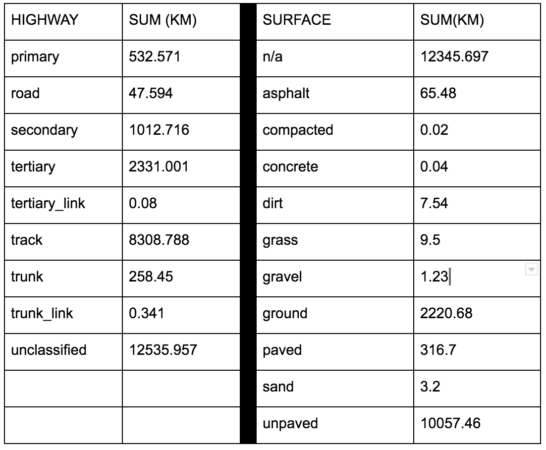
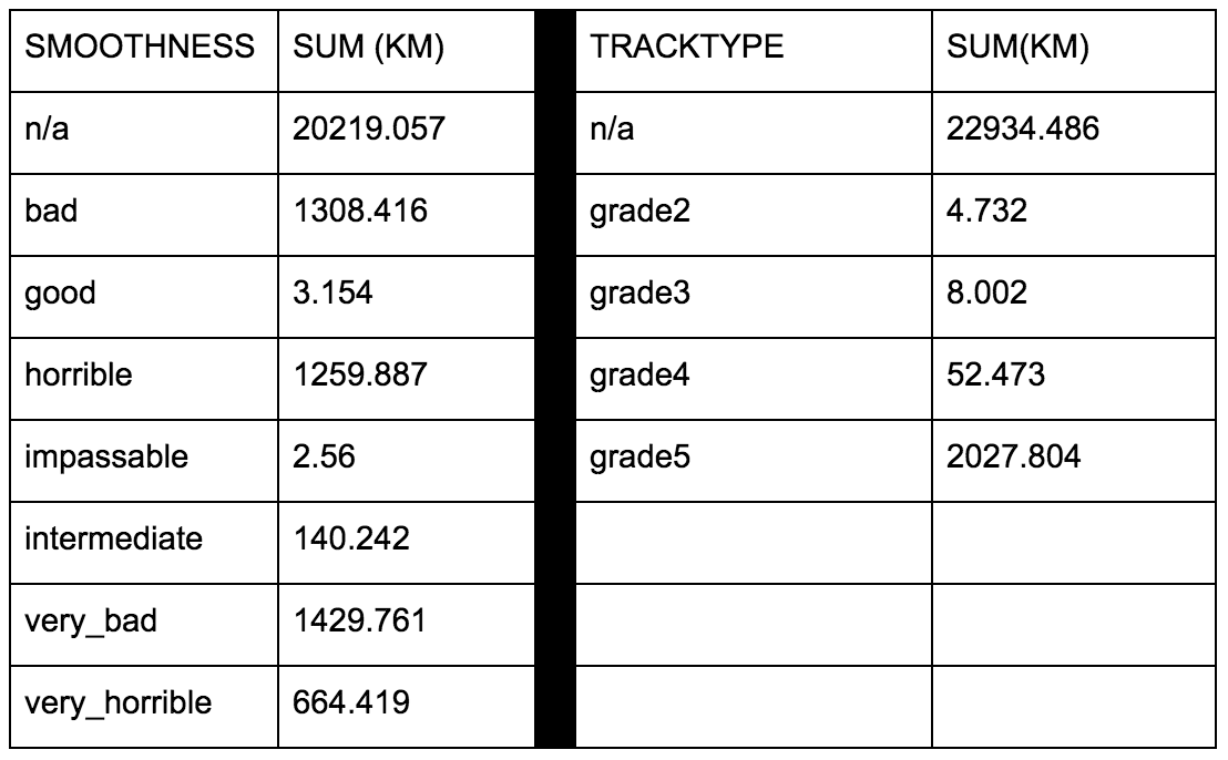
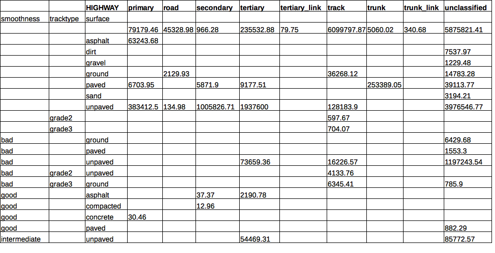
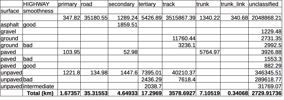
Analysing our data with GroupStats, we discovery the following situation:
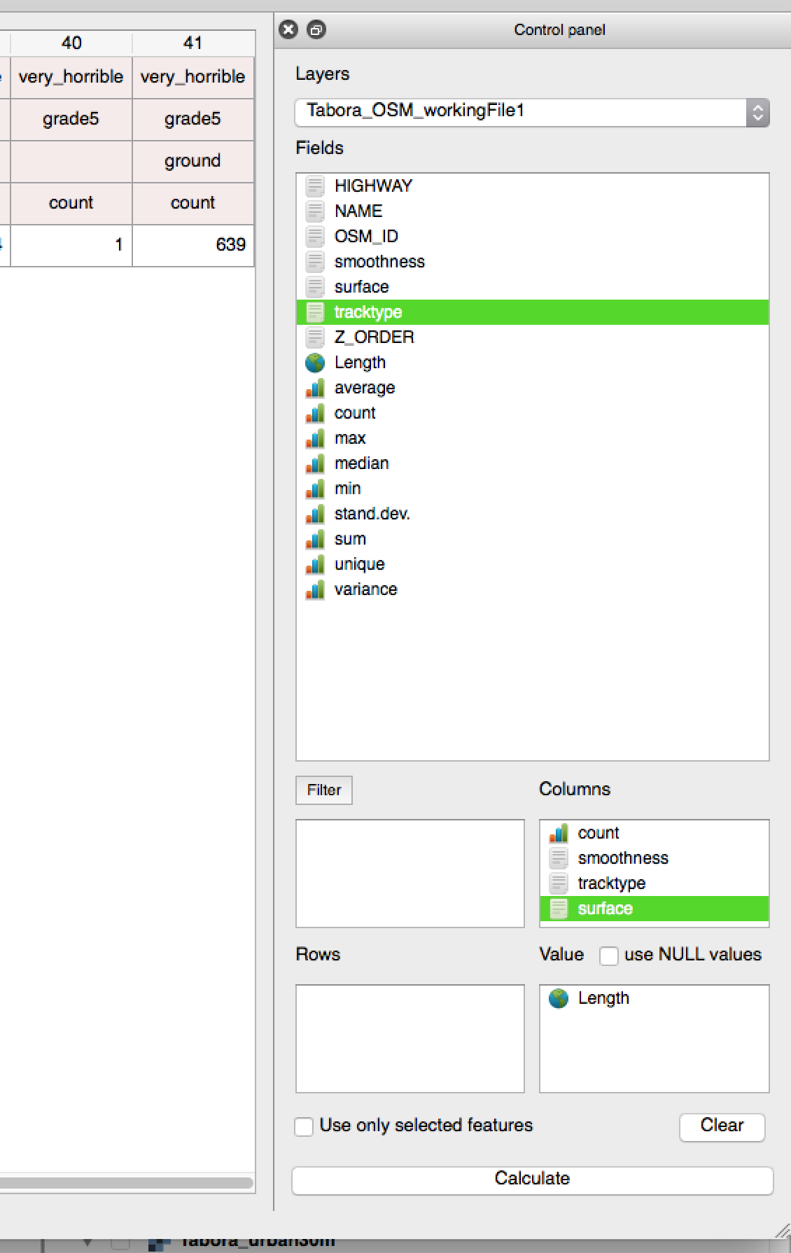
GroupStats is a plugin for easy calculation of statistics for features in a vector layer. The plugin has a control panel that allows the user to make calculations (as in our example, length) for specific group features, as can be seen in attached file 1.
A look at the complete dataset tags shows that we can find any kind of combination of the tags we are interested in. We can observe that, for our test dataset, we have 100% the HIGHWAY tag completed for all roads segments.
Continuing the analysis, with consideration to the definitions given by the OSM when assigning the specific values, we will proceed in mapping the correspondence. And so, giving the tags descriptions and the definition of a road in “good or fair condition in rural areas”, we have considered the following mappings:
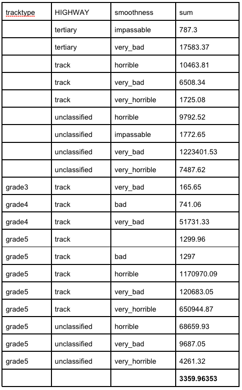
Next, we will clean the roads dataset of the categories that we have excluded, regardless of the highway=* value. Using GroupStats, we measure that we will exclude from RAI calculation. The filter GroupStats must be done by "smoothness" = 'very_bad' OR "smoothness" = 'very_horrible' OR "smoothness" = 'impassable' OR "smoothness" = 'horrible' OR "tracktype"='grade4' OR "tracktype" = 'grade5' and it will find 3082 matching features, with a total length of 3359.96 KM.
The spatial distribution of the roads eliminated from our analysis is presented in the map below:
After a quick glance, we can see that a significant central rural area is served by the roads with a too poor condition to be included in the RAI calculation.
Further on, we will work with a road layer that has been cleaned of the roads that are not in good condition. To do that, select in the attribute table using the following expression ["smoothness" = 'very_bad' OR "smoothness" = 'very_horrible' OR "smoothness" = 'impassable' OR "smoothness" = 'horrible' OR "tracktype"='grade4' OR "tracktype" = 'grade5'] and then delete the selected features.
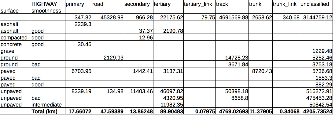
Running GroupStats, we discover the following situation for Tabora county, with respect to road condition accepted in the RAI calculations:
The next step in preparing the road dataset resides in solving the irregularities related to the road network available. With consideration to the RAI calculation, to have a correct topological road network is desirable, but not a condition. As OpenStreetMap is an open collaborative mapping project, there is a high possibility that datasets collected have all sorts of inconsistency. In the following processing steps, we are aiming at identifying and correcting these inconsistencies as to eliminate as much as possible artificial results for RAI.
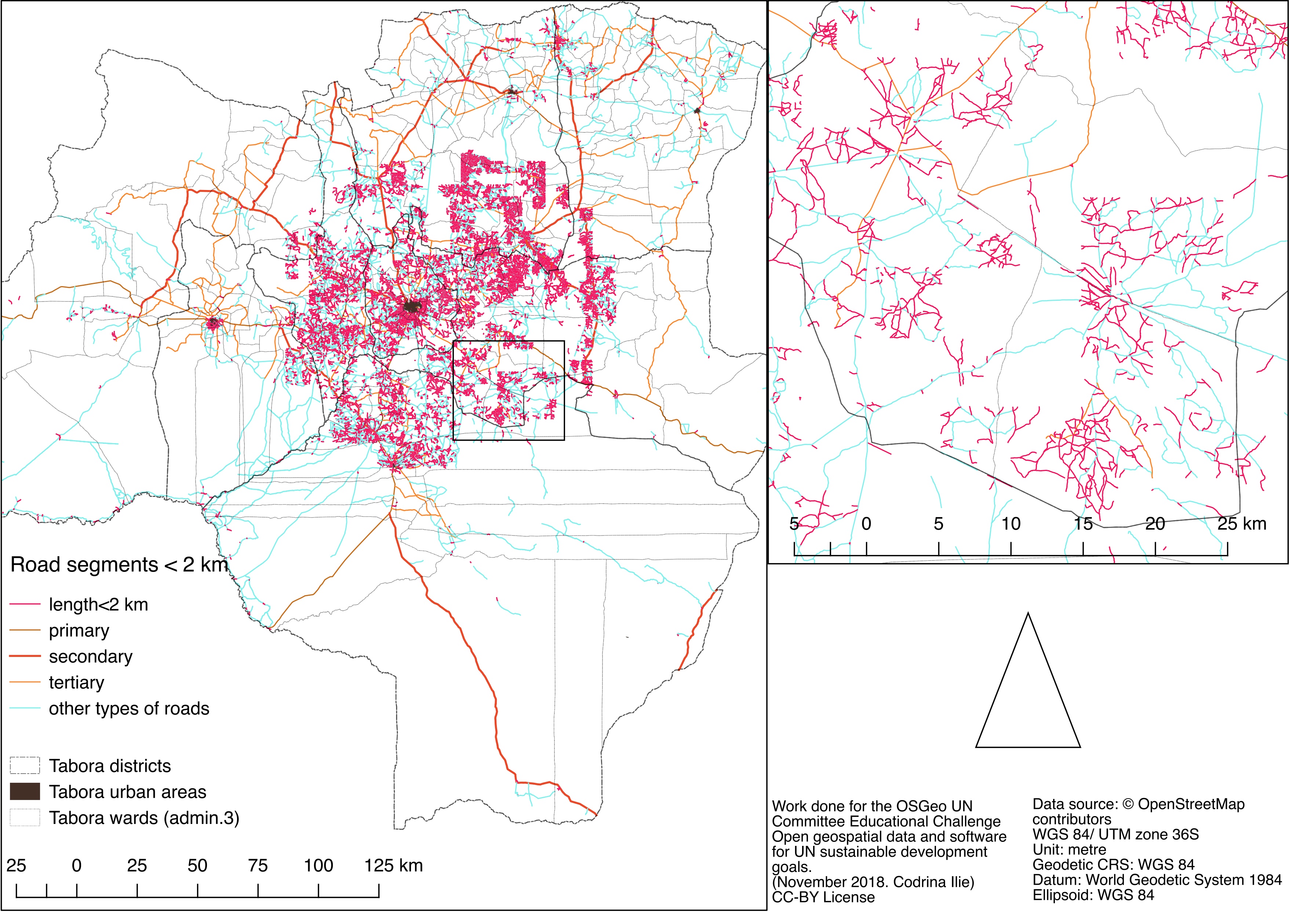
One situation to resolve is when we have segments with shorter lengths that are further away from any other connected road by at least 2 km. Why would this situation yield artificial values for RAI? Because even if rural population has access to such a road in good conditions it offers no real connectivity, it gets them only so far. Before proceeding, let us analyse the current situation: identify the percentage and spatial distribution of segments shorter than 2 km. As we can see in the attribute table, the road dataset for our exercise has 21811 features. After filtering, we identify 19709 segments that are shorter than 2km.
Filter the attribute table by "length_m" < 2000 and then run GroupStats to get a sense of your data.
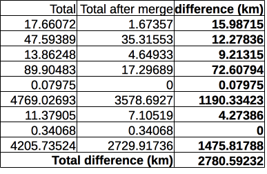
However, by looking at the geometry, we can see that a significant part of these short segments are actually completing the longer road segments. Thus, we need to connect all these segments, in order to be able to delete the features that are shorter than 2km AND not connected to any other road feature. Thus, we need to unite all road segments that are connected. As mentioned before, in our study crucial is the road network and not the topology. To do this, we will use a QGIS plugin, MergeLines. After running MergeLines, we are left with 13590 features, out of which 11298 are shorter than 2 km.
By comparing the numbers, we can see that running the MergeLines plugin represents a significant cleaning of the road dataset, with respect to RAI calculation. Almost 3000 km were road segments shorter than 2 km and would have increased the buffer calculation time artificially.
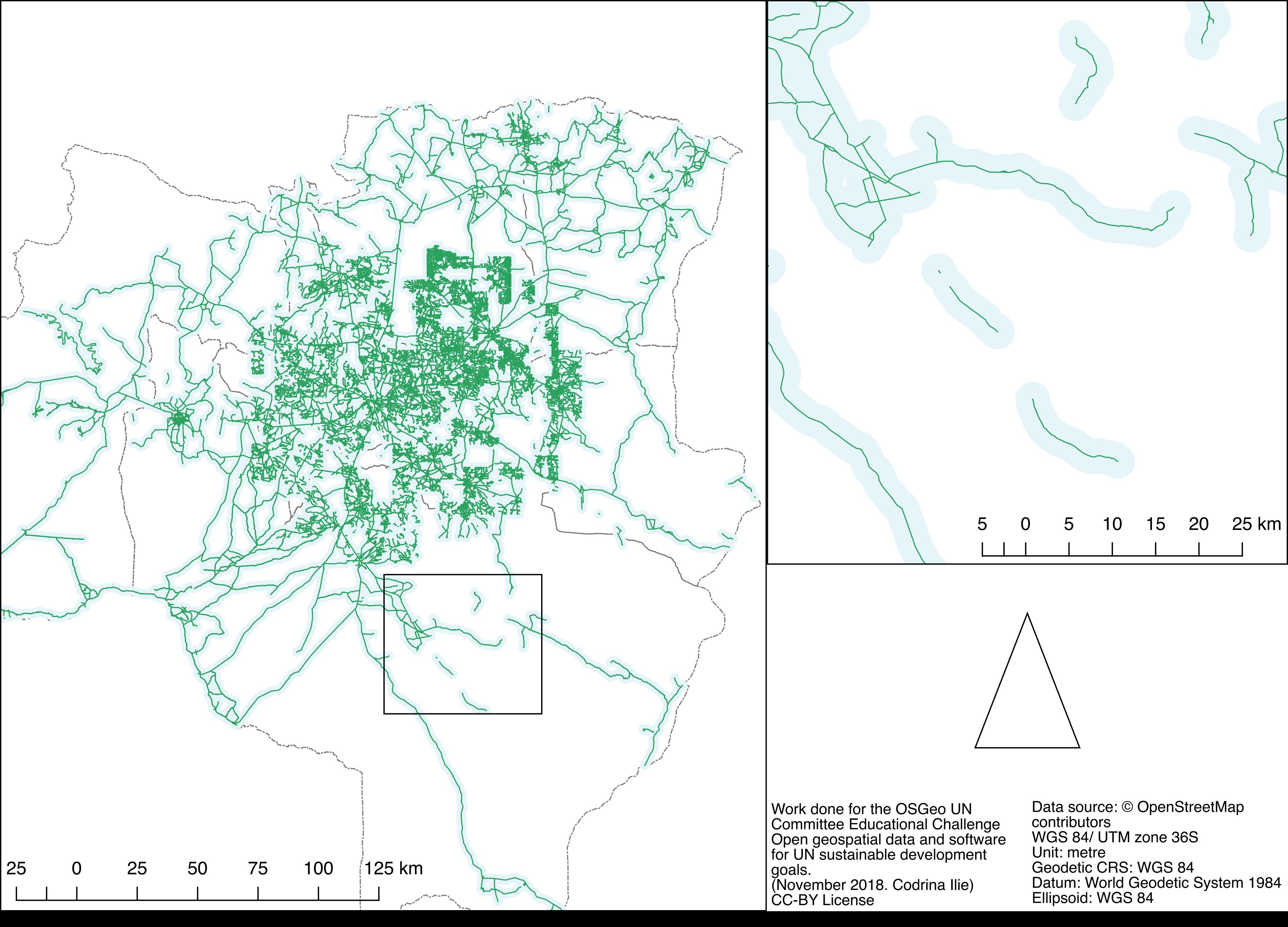
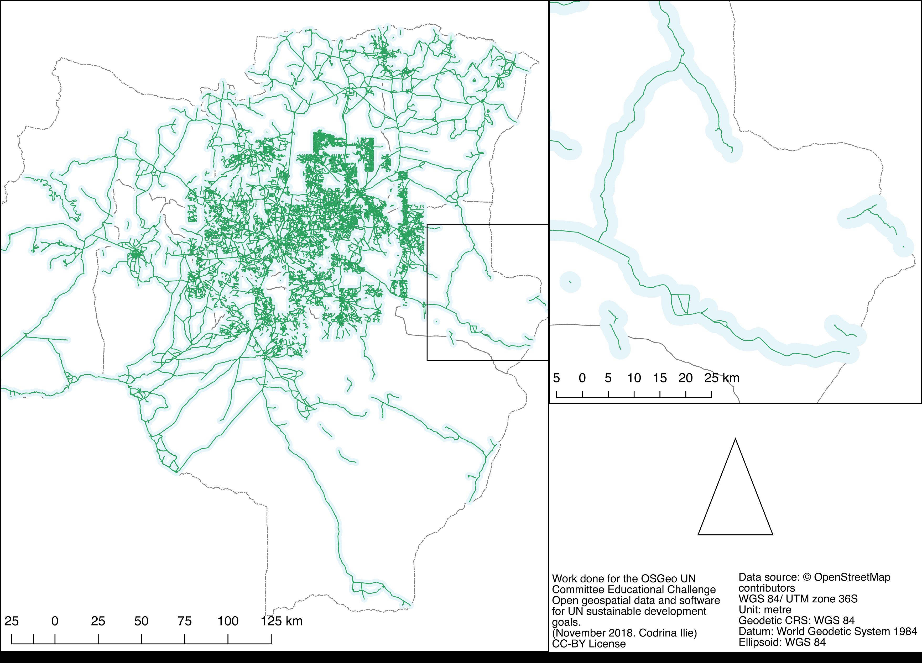
Next, we will create the 2km buffer zone around the road network. We need to identify whether there are any buffers disconnected from the network buffer. Such a case would indicate that again, there are roads in good or fair condition, that are not connected to the main road network, thus including into the RAI calculation would offer an artificial result, as it can be seen in the map below.
Before deleting the unconnected buffers, we will check to see whether the corresponding roads are not on the border. In this case, we decide not to remove them because, they might be connected to roads outside the Tabora county.
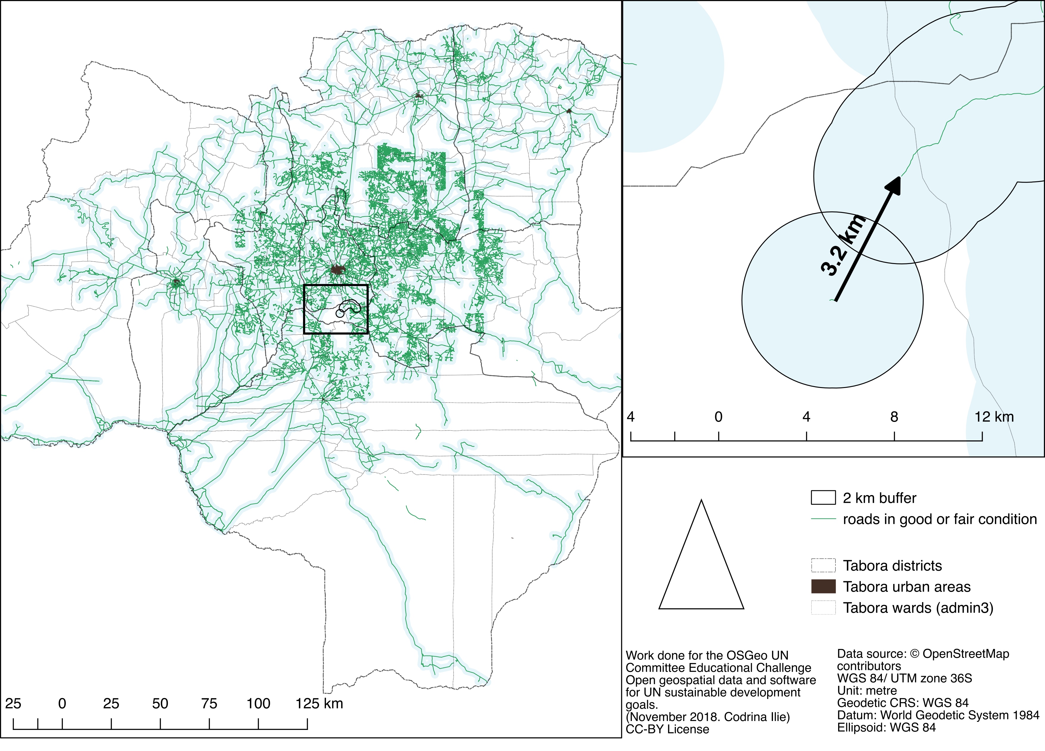
After deleting the disconnected buffer zones, we can identify a new situation that may lead to an artificial result for RAI. As shown in fig. 18, the issue can occur when we have 2 disconnected road segments that have overlapping 2km buffers and yet, the distance that one must walk from segment A to segment B is between 2.01 km and 3.99 km. Hence, the buffer should not include this area.
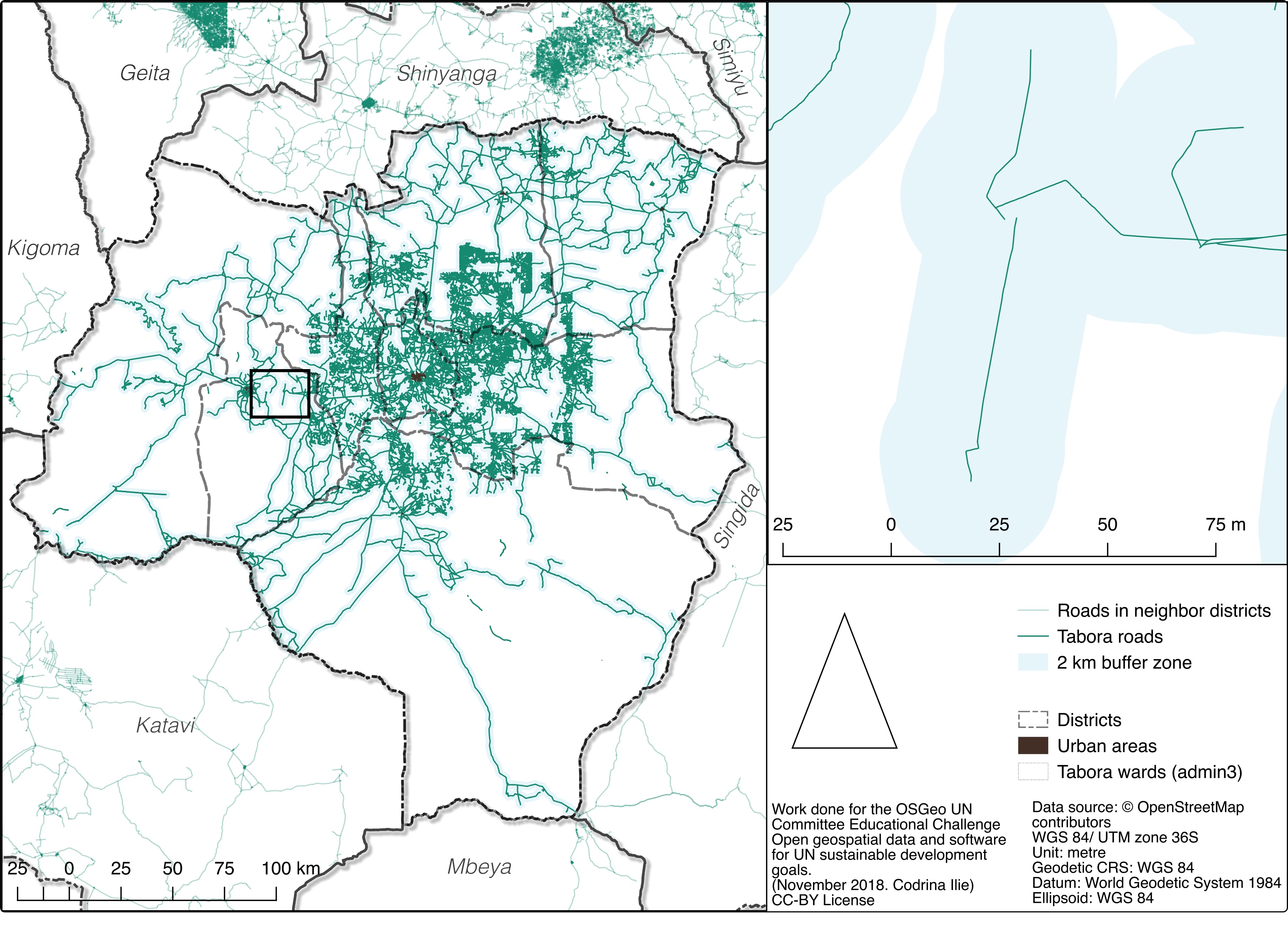
Why not just delete the unconnected segments? Because there are such road segments that would be in the 2km buffer from the road network but stretch beyond the buffer, so if we were to delete all together, we would lose the buffer region of the unconnected segment. This case is exemplified in fig. 19.
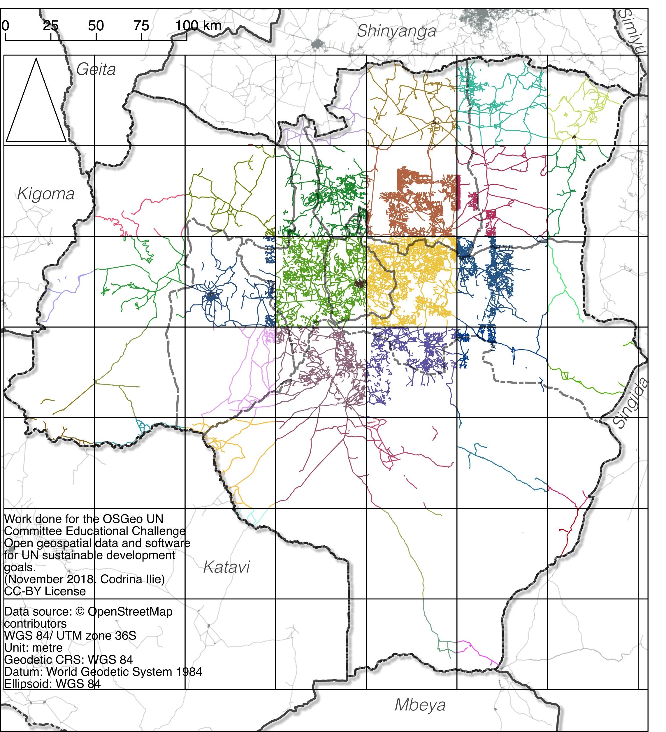
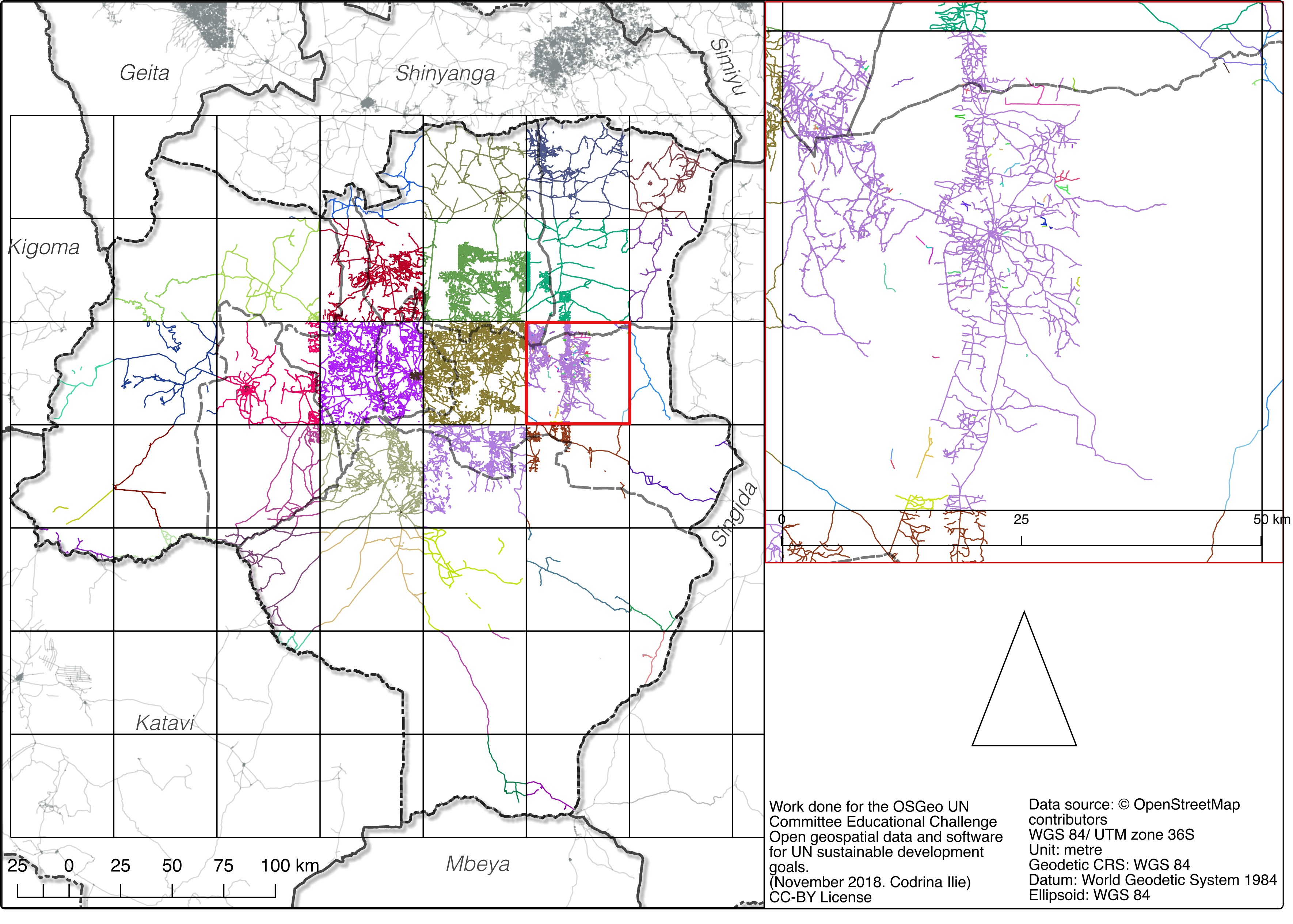
To overcome this issue, we will identify all connected segments of the road and create a 2km buffer zone for the entire network. As our dataset is substantial (over 13000 features), we will split all vectors by a 50X50 grid. [Vector]-->[Research tools]-->[Vector grid] - creates vector grid with specific extent and cell size; [Vector]--> [Geoprocessing Tools] --> [Intersection] - splits the road dataset by each grid cell; [Vector]--> [Data Management Tools] --> [Split vector layer] - creates a road layer for each grid cells.
Now that we have prepared the road dataset, we will run the script (by Jochen Schwarze) that creates networks, by merging adjacent lines. The script produces a new dataset from the input data with an attribute “subnet” that contains an incremented ID for each subnetwork created.
[Vector]--> [Geoprocessing Tools] --> [Dissolve] - the roads that all connected will be dissolved into one feature - we will run the algorithm in batch processing mode. [Vector]--> [Merge Vector Layers] - we merge all resulting layers into one road dataset. [Vector]--> [Dissolve by attribute value - subnet] - thus we will have one geometry for each subnet [GroupStats] - will be run on the Dissolve_merged dataset, because we want to extract how many road segments are in each subnet, as well as total length. The GroupStats must be configured as:
- rows=subnet /value=count,length #to count all unique segments in each subnet
- rows=subnet / value=sum,length #to calculate lengths for each subnet
Using LibreOffice, we will analyse how the road network for Tabora county looks like. We are attempting to identify road segments that can lead to artificial results of the RAI indicator.
[Layer] --> [Add] --> Delimited text layer -inserting the table created in the previous step, so we can see a spatial distribution with respect to the number of segments for each subnet, as well as by length.
Select the [dissolved_by_subnet] layer --> [Properties] --> Join - here we join the attributes calculated (segments count, sum of subnet length) to the geometry
Select the layer after joining the new attributes --> [Export..] - saving a new file as the join operation is valid only within the project.
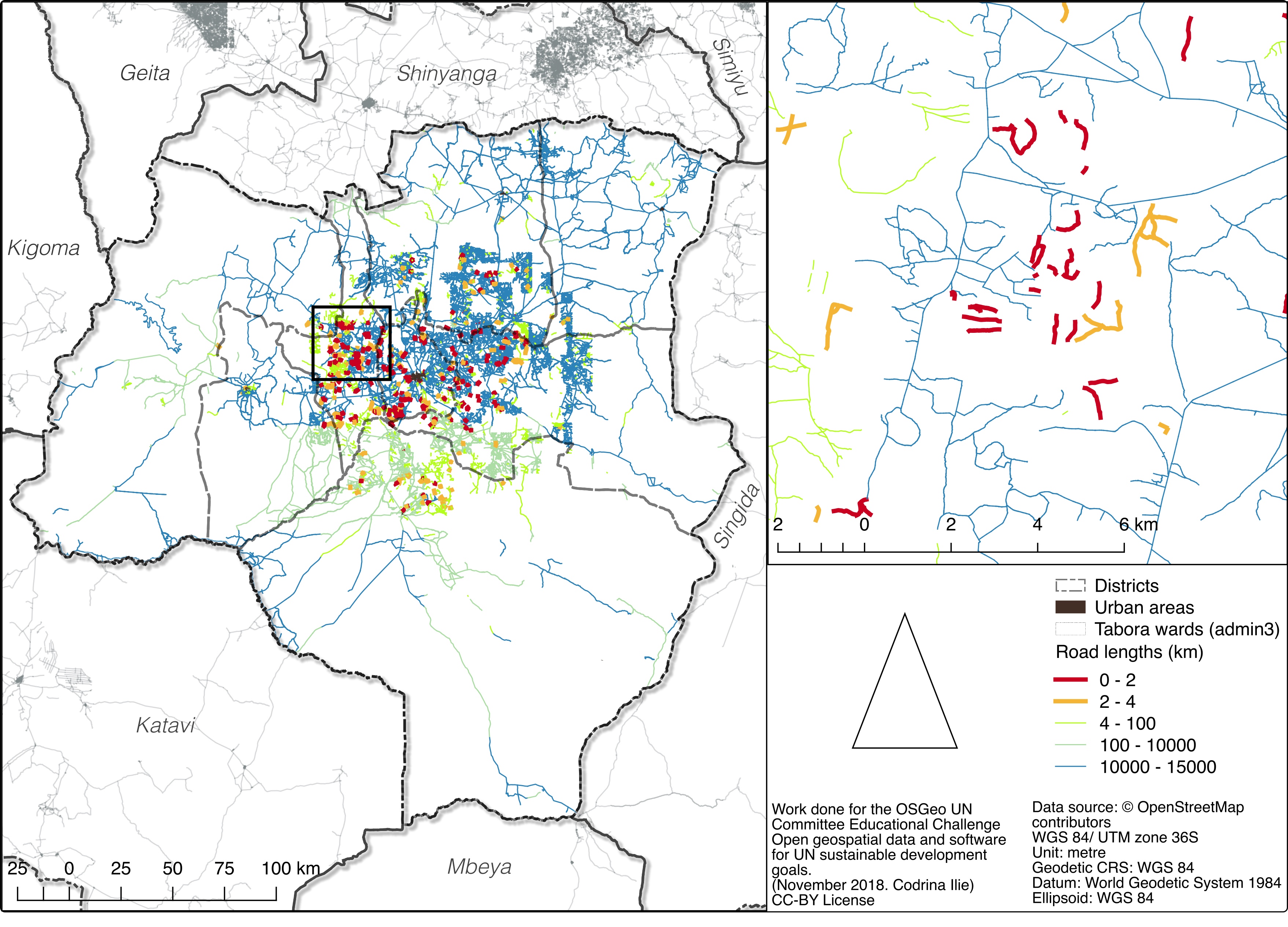
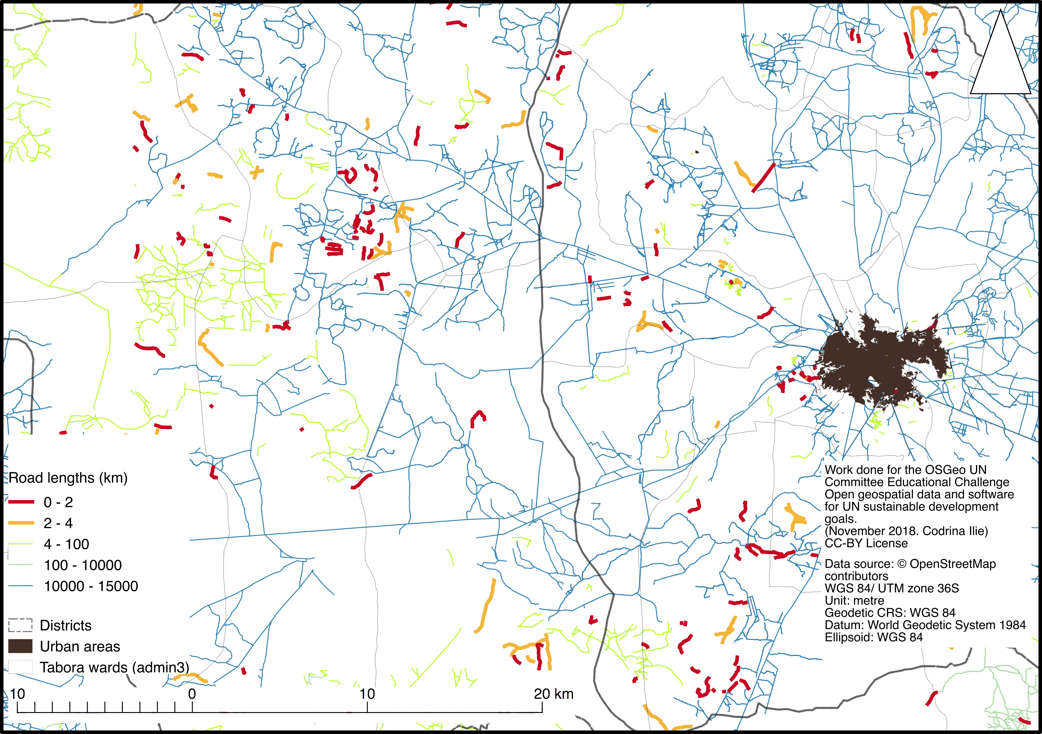
A quick analysis of the spatial distribution shows that the short road segments do not represent small disconnected parts of the road network, but rather disparate segments that do not bring a significant improvement to the road network (fig.22, fig.23).
To clean the road network in preparation for the 2km buffer calculation, we will eliminate the roads that have 1 or 2 segments, with a total length below 2 km. Now, we calculate the corresponding 2km buffer for the cleaned OpenStreetMap road network in a good condition. [Vector]--> [Geoprocessing tools] --> [Fixed distance buffer] (lengthy operation!)
Calculation of the Rural Access Index
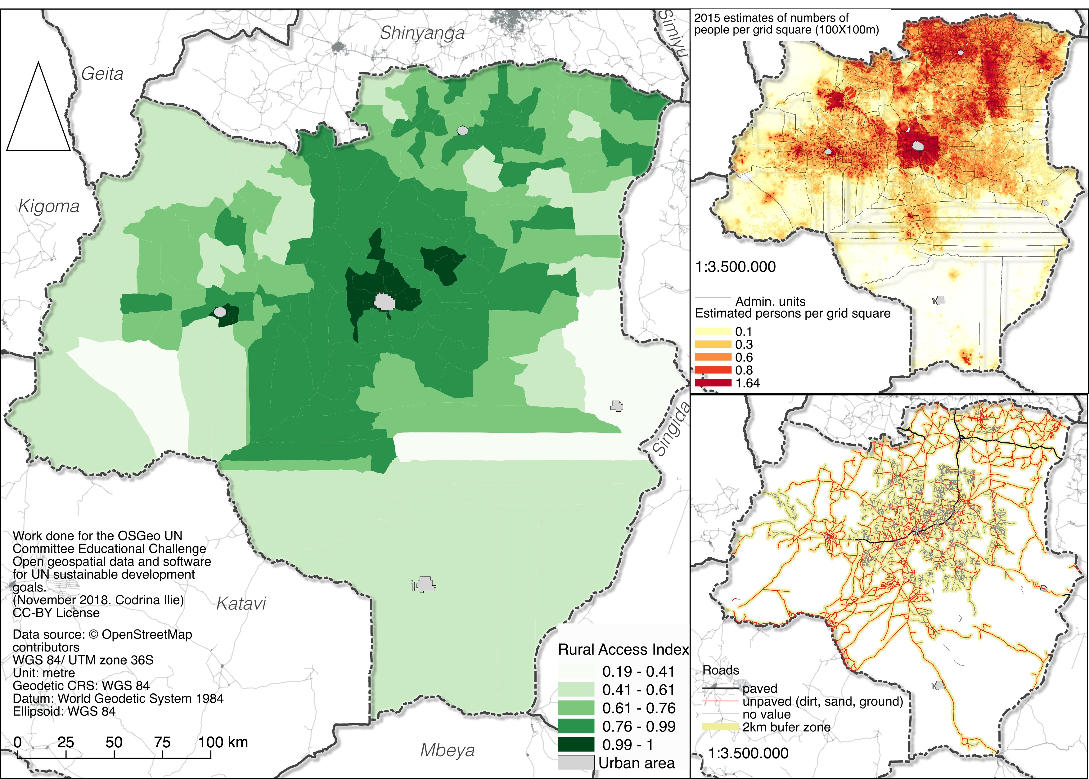
The provisional new RAI is the share of the population who live within 2 km of an all-seasons road. As we have prepared the datasets for population number, rural and urban areas, road network and road condition, we can calculate the indicator showing the number of people included - Rural Access Index.
Next, we will continue with the final series of data processing, that have already been encountered in this material.
[Vector]--> [Geoprocessing tools] --> [Clip] - we will clip the buffer zones by the administrative unit layer, as we will report on the number of rural population who live within 2 km of an all-season road by administrative unit level 3 - wards.
[Raster] --> [Zonal statistics] - we extract for each 2km buffer zone of each administrative unit, the number of people living in rural areas.
The zonal statistics functionality provides the user with the opportunity to extract using a vector mask (in our case the 2 km buffer area) from a raster the following statistics on the selected band:
- Count: to count the number of pixels
- Sum: to sum the pixel values
- Mean: to get the mean of pixel values
- Median: to get the median of pixel values
- StDev: to get the standard deviation of pixel values
- Min: to get the minimum of pixel values
- Max: to get the maximum of pixel values
- Range: to get the range (max - min) of pixel values
- Minority: to get the less represented pixel value
- Majority: to get the most represented pixel value
- Variety: to count the number of distinct pixel values
For our specific exercise, we will use Sum. To facilitate working with the dataset, we will round up to an integer for the number of people in each buffer zone.
[Vector] --> [Geoprocessing tools] --> [Clip] -before proceeding to RAI calculation, we will clip the buffer vector layer by the boundaries of the administrative units level 3.
[Vector] --> [Geoprocessing tools] --> [Difference] - so we can extract urban areas from the clipped buffer zone.
After these small processing chains, we have the 2 main layers we will use for calculation of RAI for Tabora:
- vector layer - Tabora administrative units level 3 with population number
- vector layer 2 - 2 km buffer zone for all-seasons Tabora road network, with population number for each buffer segment within each administrative unit.
The last step is to add the sum population values of the total buffer zone for each administrative unit level 3 and then divide the rural population within the buffer area by the total rural population. We do that within the [Properties] of the Administrative units level 3 vector layer [Joins] --> [join attribute values] from the 2 km buffer zone by the name of the administrative unit.
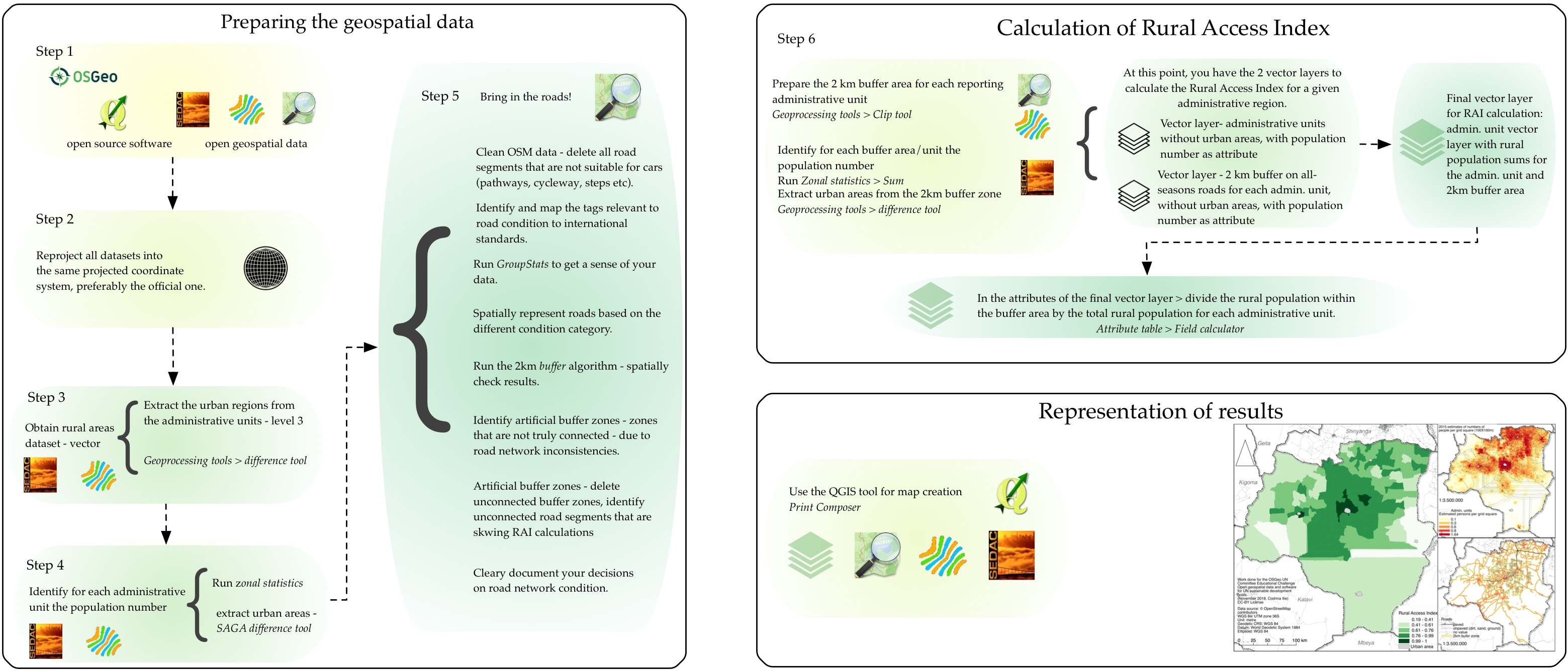
We have enclosed all steps of the processing chain detailed above in a conceptual schema of the workflow necessary to calculate the Rural Access Index using open data and open source software.
Geospatial data representations
Although, it might not always be considered as such, a significant aspect of any study, be it geospatial or not, lies in the representation of results. There are well known rules and guidelines in any type of domain and the geospatial one is no exception. Most prevalent representations come in the form of static or dynamic maps, cartodiagrams, graphs developed using various solutions, largely visualisations that are closely related to the spatial dimension of the data. The geospatial open source solutions ecosystem has reached an advanced level that accommodates the creation of highly professional maps, diagrams be they static or interactive, on paper or online. For the visualisation of the Rural Access Index results for Tabora county, we used QGIS capabilities. With the third major release of QGIS - QGIS 3.X - significant developments have been achieved, yet one crucial improvement lies in the advancements of the map composer engine. There are sufficient online and offline resources that present complete tutorials on how to use the Map Compose/Layout functionality, so we consider there is no need to duplicate already existing work. However, we are including in this material the two map templates created and used to make all representations in this material.
Known limitations of the material
The scope of this material is to show that we have entered in a time when using FOSS and open data we can initiate complex analysis allowing understanding of various facets of our environment. Works in this direction are already underway with a high focus on the knowledge we can extract from satellite imagery that have an open data policy, such as the Landsat or Copernicus programs. These works translate into global initiatives such as the Global Forest Watch or Geo Wetlands Initiative and so many more. Yet, we must not underestimate the power of what collaborative open mapping efforts can bring to our knowledge ecosystem and the OpenStreetMap project is a successful exemplification of that. Of course, one must not overlook matters related to the quality of data when it comes to the open collaborative environments, but as we have proven through this material, they provide a very good starting point that must not be neglected. As done in this study, careful analysis on understanding the datasets we are working with is crucial for eliminating as much of artificial errors of the final results as possible. Such decision is as the one we made, to eliminate roads that are shorter than 2 km and don't have more than 2 segments that would have given an artificial value of the Rural Access Index in a multitude of situations, as we presented. Nonetheless, we are aware that this decision might have lead to delete segments of roads in good condition that would be viable in the index calculation. It was a compromise that we acknowledge, after the analysing the data. Yet, it must be highlighted that this material is a first step to calculate a Sustainable Development Goal indicator, when official data is not available. Thus, in a specific case a more thorough and manual inspection of the open datasets is highly recommended.
When it comes to software, FOSS is a stable choice as it has reached a maturity level that covers all sections of a geospatial analysis, from storing, to processing to visualization, be it online or offline, dynamic and interactive or static. For our material we have used a very popular GIS open source solution - QGIS 3, but it must be highlighted that it is by far the only solution. Most, if not all steps in the processing chain we made can be accomplished using other open source solutions, as well. Our choice to use QGIS was based on the idea of using an outright, intuitive and user friendly framework.
