Training Material for UN Open GIS Spiral 3

1. General Info

The OSGeo UN Committee promotes the development and use of open source software that meets UN needs and supports the aims of the UN. Following a meeting between OSGeo Board of Directors and the UN GIS team at FOSS4G in Seoul, Korea in September 2015, the Committee has mainly worked on the UN Open GIS Initiative, a project “...to identify and develop an Open Source GIS bundle that meets the requirements of UN operations, taking full advantage of the expertise of mission partners including partner nations, technology contributing countries, international organisations, academia, NGOs, private sector. The strategic approach shall be developed with best and shared principles, standards and ownership in a prioritized manner that addresses capability gaps and needs without duplicating efforts of other Member States or entities. The UN Open GIS Initiative strategy shall collaboratively and cooperatively develop, validate, assess, migrate and implement sound technical capabilities with all the appropriate documentation and training that in the end provides a united effort to improve the effectiveness and efficiency of utilizing Open Source GIS around the world.” (more details at [1]).

OSGeo UN Commiittee called proposals for developing open geospatial educational materials (more details at [2]) as a part of the activities in the OSGeo UN Commiittee. Silvia Franceschi (HydroloGIS) was selected as a winner for "Educational Challenge 2". This document is the result of the challenge 2.

1.1 Purpose of this document

This educational material is designed as a step-by-step software learning guide for geo-analytic library called "uDig Processing Toolbox".

Geo-analytic functions in the 'Processing Toolbox' library are divided into 4 categories. First General Tools are to support I/O, visualize, primitive geometry functions such as extract, clip, aggregate and dissolve. Second, Spatial Statistics Tools are to provide geo-statistical analysis functions such as Ordinary Least Squares s(OLS). Third, Raster Tools are to support raster data analysis functions such as Radial Line of Sight.

This tutorial contains the description of the usage of some commands for environmental analysis of raster and vector data with the uDig Processing Toolbox. The purpose of this quick start document is to introduce the user in the use of the algorithms contained in the Processing Toolbox of uDig for environmental analysis in particular related to ecology and ecosystems identification.

In this tutorial, you will perform the following tasks:

• preliminary operations

• raster data analysis

  • NDVI

  • DTM and DTM derived data

• vector data analysis

  • density

  • proximity analysis

  • assign attributes

  • interpolation on raster

1.2 Target Audience

The primary target audience is professionals who needs geo-statistic functions.

1.3 License

This educational material was written by Silvia Franceschi and Andrea Antonello (HydroloGIS) with the menthorship of HaeKyong Kang of the Korea Research Institute for Human Settlements and Minpa Lee of MangoSystem, within the project of collaboration between the OSGEO foundation and UN institute under the framework of the UN OSGeo Challenge. It is distributed according to the CREATIVE COMMONS deed: Attribution - NoDerivs 2.0. According to this license type you are free to:

• copy, distribute, display and perform the work
• make commercial use of the work

Under the following conditions:

• you must attribute the work in the manner specified by the author or licensor
• you may not alter, transform, or build upon this work.

For any reuse or distribution, you must make clear to others the license terms of this work. Any of these conditions can be waived if you get permission from the copyright holder.

Your fair use and other rights are in no way affected by the above. This is a human-readable summary of the Legal Code (the full license) that can be consulted at: website.

2. Preparation

2.1 uDig and "Processing Toolbox"(uDig plugin for geo-analysis library)

2.1.1. Install uDig SW

You can download uDig for Windows 64bit at udig-2.0.0-SNAPSHOT.win32.win32.x86_64.exe. Other uDig versions are accessible at uDig webpage .

2.1.2. Load "Processing Toolbox" plug-in

Please keep the repository information for Processing Toolbox plug-in.
*Name: Processing Toolbox for uDig
*URL: http://www.mangosystem.com:8080/s2toolbox_updates

Now, lets’ load the Processing Toolbox into uDig.
Step1. Set a location of repository for Processing Toolbox plug-in.
[Help] --> [Find and Install] (Figure2): Install/Update window will pop up (Figure3) --> Click ‘Search for new features to install’ --> ‘Next’ button: Install window will pop up (Figure 4) --> Click ‘New Remote Site’ button à put repository Name and URL --> Click ‘OK’ button (Figure 5) --> Next button (Figure 6)

Step 2. Agree Feature License (Figure 7)
Step 3. Loading plug-in (Figure 8) à Install all (Figure 9) à Restart (Figure 10)
Step 4. View Processing Toolbox on uDig (Figure11- Figure 13)

2.2 Download a dataset for geo-analysis

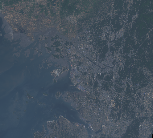
First of all get (or download) the Processing Toolbox dataset at processing_toolbox_tutorial_dataset.zip and unzip the content directly in a folder on your PC. The dataset covers an area around the city of Seoul in South Korea and contains three different type of information:

• Landsat8 images LC08_L1TP_115034_20180721_20180731_01_T1.tar.gz: unzip and untar this file to obtain a folder containing all the 11 available bands of the Landsat8 images in WGS84/UTM zone 52N coordinate system EPSG:32652.
• Aster Digital Elevation map (DTM at a resolution of 20 m) 20180814093648_947847400.zip: unzip this file and consider the geotif in LongLat WGS84 coordinate system EPSG:4326.
• Open Street Map vector dataset south-korea-latest-free.shp.zip: unzip this file and consider the 18 shapefiles downloaded from the OSM website. The files are in LongLat WGS84 coordinate system EPSG:4326.

2.3. Set UDig : New Project and New Map

First of all you have to prepare a dedicated Project and Map in uDig. In order to obtain correct results of the processing tools it is recommended to convert all the dataset in a unique coordinate reference system. Since for the current use case the data have different coordinate reference systems, we choose to work with metric coordinate reference system UTM zone 52N, EPSG: 32652.

Before starting with the analysis please do the following preliminary operations:

1. open uDig
2. select the Catalog view from the available views of the main application (usually this is placed in the lower part of the main window)
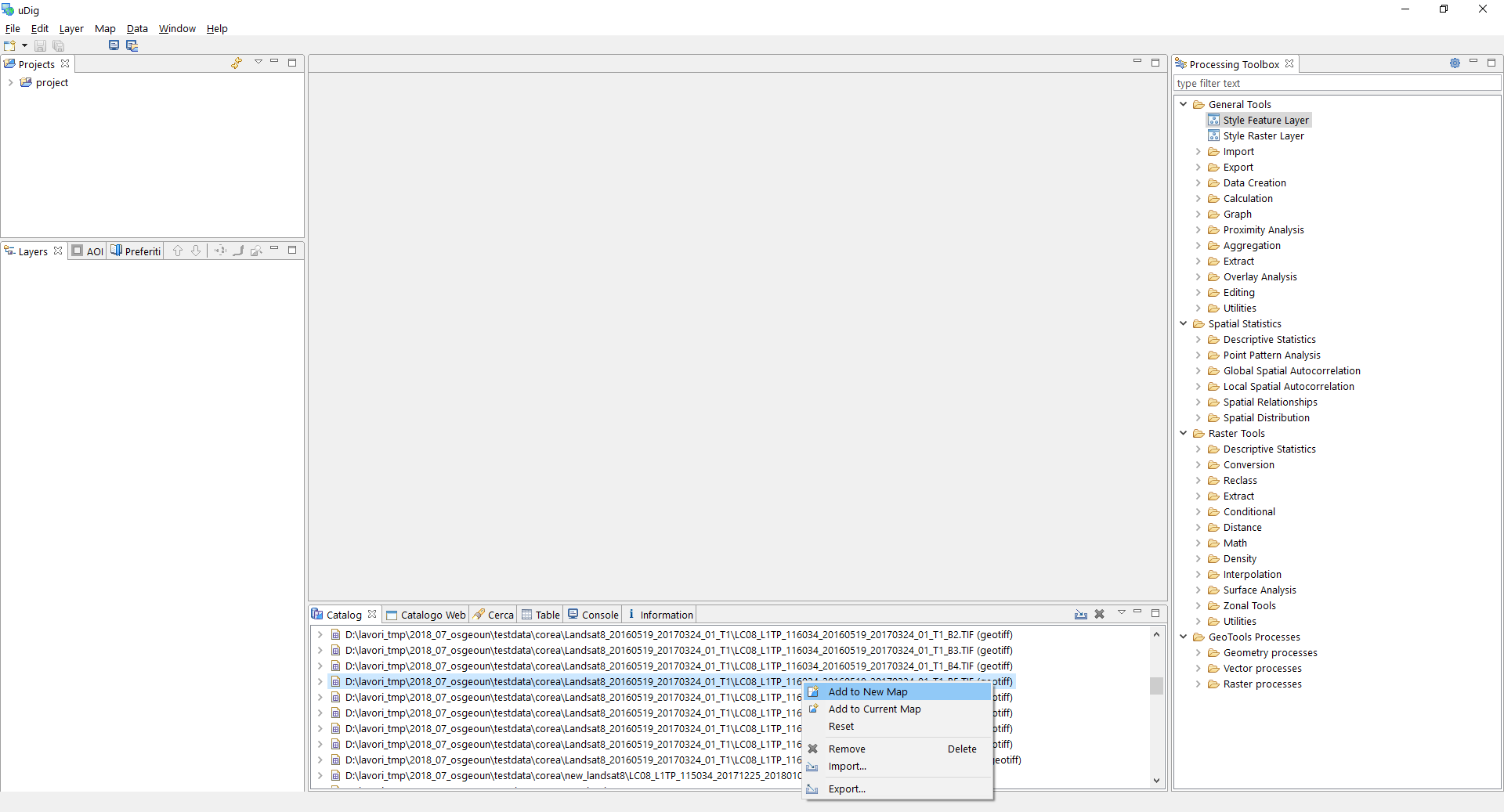
3. drag and drop the files of the Landsat8 images band 4 and 5, the DTM and the vector layers of landuse, natural points, roads and water ways from your File Manager into the Catalog view
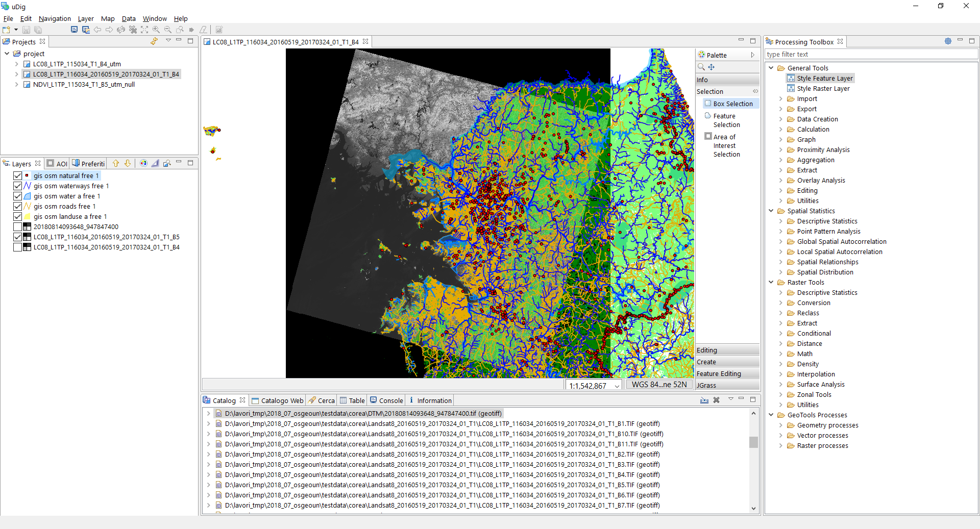
4. right click on the Landsat8 geotif and select Add to New Map or drag and drop it in the Layers view: this should open a new Map view with the coordinate reference system of the selected data source, in this case WGS84/UTM zone 52N (please take care that this is the projection of your working View)
5. drag and drop the other files directly in the Map view or in the Layers view to visualize them all in the map.

Template:Note uDig automatically reprojects the layers in the projection of the Map view, but only for visualization, the data remain in the original projection.

Figure 1. Create the Map view starting from the layer of the Landsat8 images.

Figure 2. Import of the test dataset in uDig, zoom to all layers.

2.4 Set Coordinate Reference System of the dataset

Usually we use data from different sources therefore, very often the available information are on different coordinate reference systems (CRS) and on different/widen areas. To homogenize the works and assure that all the tools work perfectly it is reccommanded (at least) to reproject all the data in the same CRS and define a working area where to clip all the data.

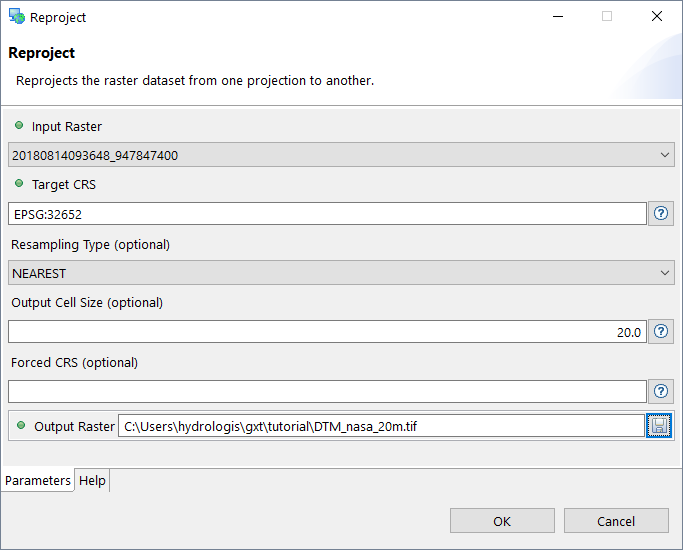
Reproject reprojects the selected layer in the given CRS. There are two different versions of the tool specific for raster and vector layers available in:

• for raster layers:

Raster Tools → Utilities → Reproject

The tool requires in input:

1. Input Raster layer: select the raster layer to reproject from the list of the raster layers available in the Map

2. Target CRS: the target CRS, you can write it in the form of EPSG:32652 or click the at the end of the line to choose how to select it:

   • CRS form current Map

   • CRS from layers → then select the layer

   • select CRS → open the standar uDig window where to select the CRS

3. Resample Type: default value is NEAREST, other options are BILINEAR and CUBIC

4. Output Cell Size (optional): the size of the output raster if different from the original

5. Forced CRS (optional): force the CRS of the input raster map to the one specified here in case the input file misses this information

6. Output Raster: the path and name of the output raster layer.

Template:Note It is important to fix the resolution of the output raster (Output Cell Size) especially with reprojection between systems using different measurement units (degree vs metric) and in any case to be sure to have squared cells in the output layer. Squared cells are mandatories if you want to use some analysis tools and in particular to use the tools of the HortonMachine library.

Figure 3. Execution of the Reproject command for the raster of DTM.

Template:Note To open the graphical interface of the commands available in the list of the Processing Toolbox double click on the name of the tool you want to run. To run the tool click on the OK button after filling all the required input in the window. To exit the tool once executed, click on Cancel. The tool will run every time you click on the Ok button.

Template:Note The output raster will be visualized all white, use the Styling System of uDig for a better visualization.

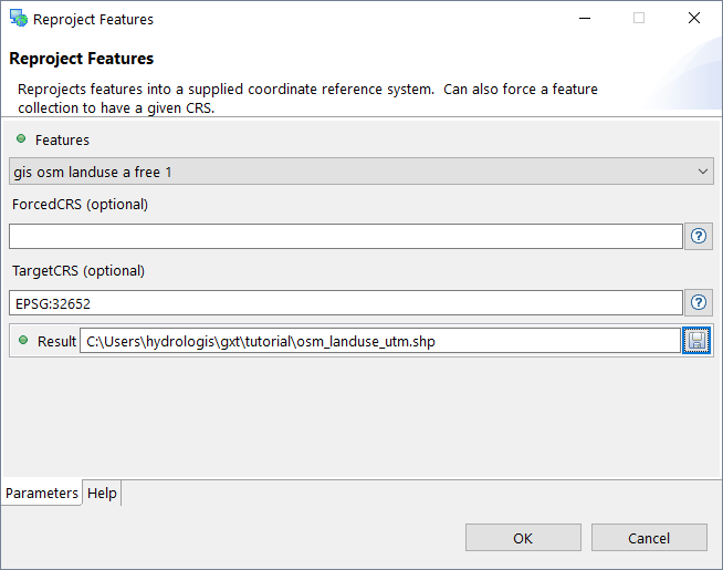
• for vector layers:

GeoTools Processes → Vector processes → Reproject

1. Feature layer: select the vector layer to reproject from the list of the vector layers available in the Map

2. Forced CRS (optional): force the CRS of the input vector map to the one specified here in case the input file misses this information

3. Target CRS: the target CRS, you can write it in the form of EPSG:32652 or click the at the end of the line to choose how to select it:

   • CRS form current Map

   • CRS from layers → then select the layer

   • select CRS → open the standar uDig window where to select the CRS

4. Result: the path and name of the output vector layer.

Figure 4. Execution of the Reproject command for the vector of the landuse.

To go on with the tutorial please reproject using the same tool as for the landuse layer also the vector layers of:

• gis_osm_natural_free_1
• gis_osm_waterways_free_1
• gis_osm_water_a_free_1
• gis_osm_roads_free_1
• gis_osm_landuse_a_free_1.

* Delete original layers after reprojecting

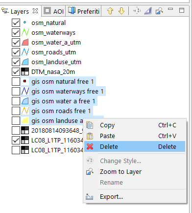
After reprojecting all the layers you can delete the original layers from the Layers view. To do this you can select all the layers or one layer at a time from the Layers view and select Delete from the context menu of the right mouse click.

Figure 5. Delete some layers from the Layers view.

2.5 Clip dataset for the next analytic process

Clip extracts the features of the selected layer for a defined region.

Before starting with the clipping we should define our working area as a polygon geometry. The standar process to do this operation in uDig is the following:

1. create a new layer: Layer → Create

2. define the characteristics of the new layer:

   • name: area_of_interest

   • attributes:

     • name: String

     • geometry: Polygon

     • CRS: UTM zone 52N (EPSG: 32684)

3. click on OK to add the new layer to the project

4. select the editing tool to Create → Create Rectangle

5. draw a rectangle in the area around Seoul (not too big but big enough to contain some of the natural points, see the picture).

The following image contains an example of the area of interest.

Figure 6. Example of the layer of the area of interest.

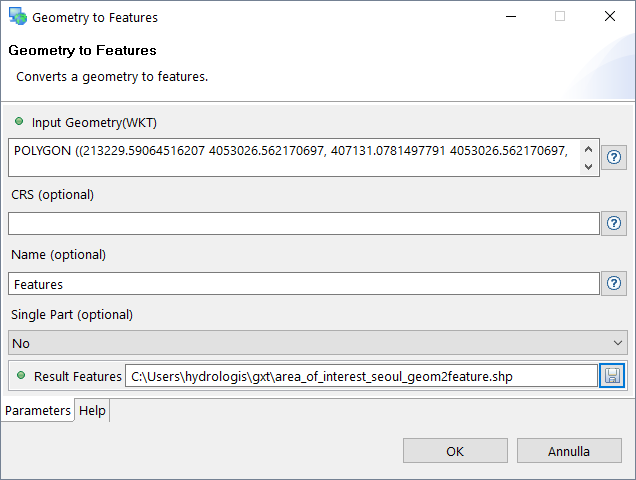
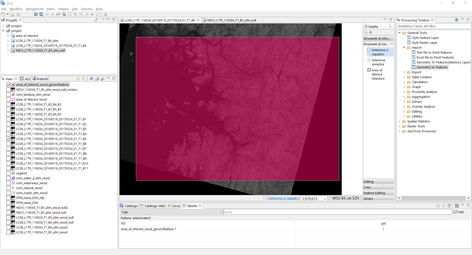
There is a new module in the Processing Toolbox developed to simplify this operation. In fact, the Geometry to Features tool can be used to automatically extract a polygon layer on the Map extent.

General Tools → Import → Geometry to Features

The tool requires in input:

1. Input Geometry (WKT): the geometry to import, click the at the end of the line to choose how to select it:

   • Point

   • LineString

   • Polygon: and then select the first option Polygon from Map’s Extent

   • Geometry from Layers…​: select the layer or the features to use to create the new layer

2. CRS (optional): the CRS of the input geometry if different from the one of the current Map

3. Name (optional): name for the features in the new layer

4. Single Part (optional): boolean variable to define if it is required to split multipart geometry to single parts, default is No

5. Result Features: the path and name of the output layer containing the new features.

Figure 7. Execution of the Geometry to Features command to extract the area of interest.

Figure 8. Example of the layer of the area of interest extracted with the command Geometry to Features.

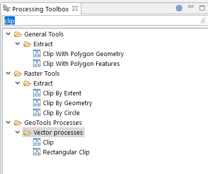
The Processing Toolbox contains some different versions of the clipping tool. You can visualize all of them just typing the word clip in the search box of the Processing Toolbox window.

Figure 9. Search for the different possibilities of clipping operations in the Processing Toolbox.

In particular we are interested in clipping both raster and vector layers and therefore we will use:

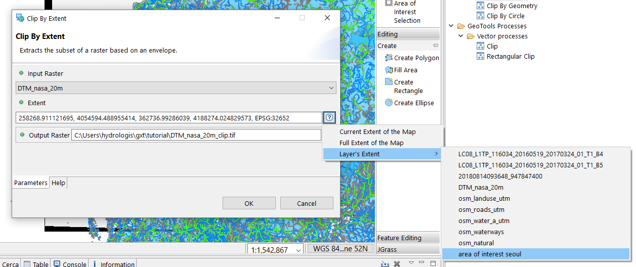
• for raster layers:

Raster Tools → Extract → Clip by Extent

The tool requires in input:

1. Input Raster layer: selects the raster layer to clip from the list of the raster layers available in the Map

2. Extent: a reference for the boundaries of the clipping area, click the at the end of the line to choose how to select it:

   • Current Extent of the Map

   • Full Extent of the Map

   • Layer’s Extent: selects the layer of the area_of_interest

3. Output Raster: the path and name of the output raster layer.

Figure 10. Execution of the Clip by Extent command for the projected raster of the DTM.

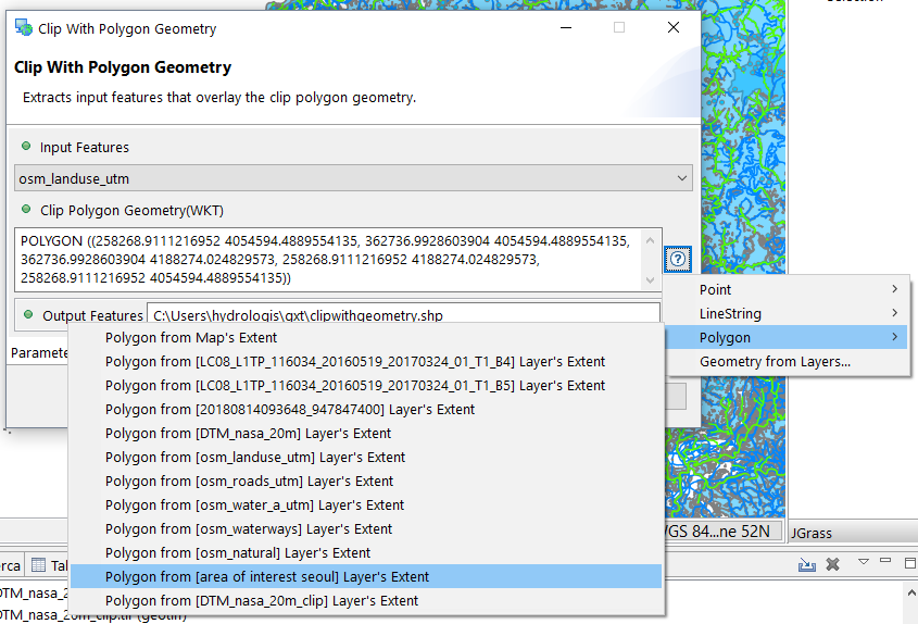
• for vector layers:

General Tools → Extract → Clip With Polygon Geometry

The tool requires in input:

1. Input Feature layer: select the vector layer to clip from the list of the vector layers available in the Map

2. Clip Polygon Geometry (WKT): a reference for the boundaries of the clipping area, click the at the end of the line to choose how to select it:

   • Point

   • LineString: selects the boundary from the area_of_interest Layer’s Extent

   • Polygon: then selects the polygon from the area_of_interest Layer’s Extent

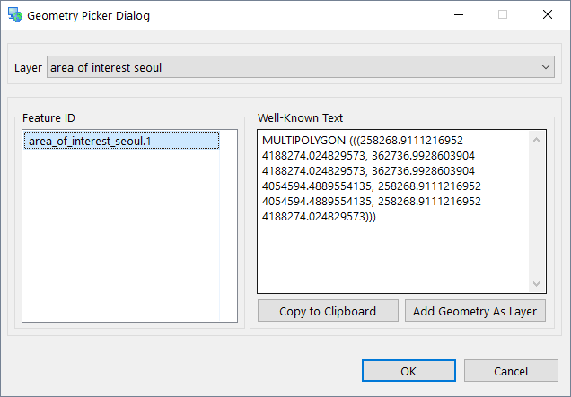
   • Geometry from Layers…​: select the layer and feature ID of the polygon to use for delimiting the new vector layer

3. Output Features: the path and name of the output vector layer.

Figure 11. Execution of the Clip With Polygon Geometry command for the projected vector of the landuse.

Figure 12. Execution of the Clip With Polygon Geometry command for the projected vector of the landuse, select the geometry picker.

To go on with the tutorial please clip using the same tools as used for DTM and landuse, respectively for raster and vector layers, also the other following layers (take care to use the reprojected ones):

• Landsat8 images of band 4 and 5: LC08_L1TP_116034_20160519_20170324_01_T1_B4.TIF and LC08_L1TP_116034_20160519_20170324_01_T1_B5.TIF
• osm_natural_utm
• osm_waterways_utm
• osm_water_a_utm
• osm_roads_utm.

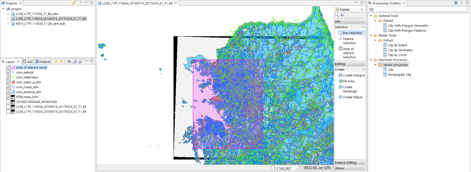
After clipping all the layers you can delete the original layers from the Layers view.

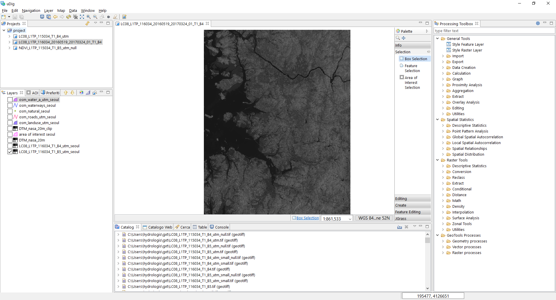
The final configuration of the application and data should be like the one in the next image.

Figure 13. Configuration of the uDig application after the preliminary operations.

SetNull sets specific values in the raster layer to assign to NoData. This tool works only for raster layers and it allows the user to set the cell with certain values to NoData (not valid). Doing this, these cells will be automatically excluded from further elaborations on the raster maps like statistical analysis or during the evaluation of spatial indexes.

Template:Note To query single values of the raster layers or to display the attributes of specific features of vector layers please use the info tool of uDig available in the Palette of the Map view.

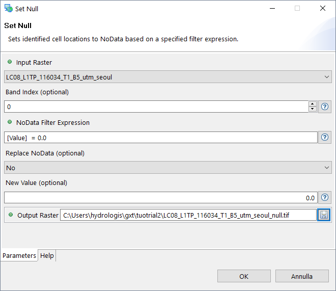
To set the value of 0.0 of the Landsat8 images to NoData you can use the SetNull tool available in:

Raster Tools → Conditional → Set Null

The tool requires in input:

1. Input Raster layer: select the raster layer of which to set the NoData values from the list of the raster layers available in the Map
2. Band index (optional): optional value of band index to use for multiple band layers, otherwise leave it at 0
3. NoData Filert Expression: expression used by the software to identify the NoData values in the layer, click on the at the end of the line to choose how to define it.
4. Replace NoData (optional): flag to identify if the tool has to work in the standard or in the opposite way, that means replacing NoData values with a valid value
5. New Value (optional): this value is required only if the Replace NoData is activated (Yes) and it represents the new value to assign to previous NoData values
6. Output Raster: the path and name of the output raster layer.

Figure 14. Execution of the Set Null command for the raster of the Landsat8 images.

In our example we have to set the value 0.0 of the Landsat8 images to NoData. This expression is very easy and can be written directly in the NoData Filert Expression as:

[Value] = 0.0

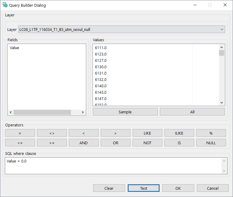
In case there is the need to use more advanced expressions to identify the values of a raster map to set to NoData it is possible to use the Query Builder Dialog integrated in the Processing Toolbox just clicking on the button and select:

• Layer: only for testing the expression directly in the Query Builder Dialog
• Fields: in case of raster layers the only field available is the Value, double click on the item in this section to add it to the query or type Value directly in the text field below
• Operators: select one of the available operators or directly type it in the text field below
• SQL where clause: the resulting SQL expression used by the software for filtering the values and assigning the NoData.

The Query Builder Dialog gives also the possibility to show in the Values section a sample or all the data contained in the selected raster layer clicking on the Sample, or for all values on All button and to Test the expression inserted clicking the specific button at the bottom of the window.

Figure 15. The Query builder options of the Set Null command for the raster of the Landsat8 images.

To go on with the tutorial please set the null values to zero using the same Set Null tool for both the raster layers of the Landsat8 images, band 4 and 5: LC08_L1TP_116034_T1_B4_utm_seoul.tif and LC08_L1TP_116034_T1_B5_utm_seoul.tif.

3. Analysis of Landsat raster images

In the field of environmental sciences lot of analysis have to be performed on raster data. In this tutorial we will consider two different kind of raster data:

1. satellite images (Landsat8)
2. digital elevation maps (DTM) and derived products.

Raster data are continuous data in the format of a matrix of cells (or pixels) organized into rows and columns where each cell contains a value representing the content of the raster. The easiest way to observe the contened values is to use a right style, but if you need some more precise information you have to analyse them. The Spatial Toolbox provides useful tools for analyzing and do elaborations of raster layers.

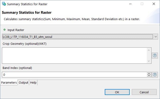
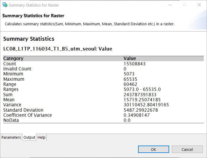
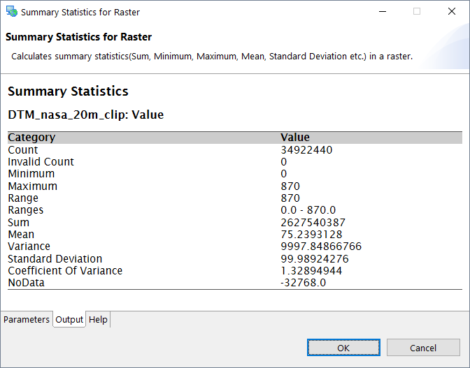
Summary Statistics for Raster is a tool which prints a summary of the main statistics of the selected raster layer. It is available in the section:

Raster Tools → Descriptive Statistics

double click on the Summary Statistics for Raster entry. The required input parameters are:

1. Input Raster layer: select the raster layer to elaborate from the list of the raster layers available in the Map

2. Crop Geometry (optional): a reference for "clipping" a custom area of the raster layer if you need to extract the information on a subset of the complete raster; click the at the end of the line to choose how to select it:

   • Point

   • LineString: selects the boundary from the area_of_interest Layer’s Extent

   • Polygon: selects the polygon from the area_of_interest Layer’s Extent

   • Geometry from Layers…​: selects the layer and feature ID of the polygon to use for delimiting the new vector layer

3. Band Index (optional): optional value of band index to use for multiple band layers, otherwise leave it at 0.

Figure 16. Execution of the Summary Statistics for Raster.

The tools evaluates the following statistics:

• Count: number of valid cells of the raster layer
• Invalid Count: number of not valid cells or unclassified values
• Minimum: minimun value of the raster
• Maximum: maximum value of the raster
• Range: the entire range of the data content in the raster layer (max - min)
• Ranges: the available ranges the data content in the raster layer in case of an elaboration on multiple geometries
• Sum: the sum of the data content in the raster layer
• Mean: the average of the data content in the raster layer
• Variance: the variance of the data content in the raster layer
• Standard Deviation: the standard deviation of the data content in the raster layer
• Coefficient of Variance: the Relative Standard Deviation of the data content in the raster layer
• NoData: the value representing the NoData cells in the raster layer.

Figure 17. Output of the Summary Statistics for Raster on the Landsat8 image of Band 5.

Figure 18. Output of the Summary Statistics for Raster on the DTM.

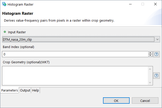
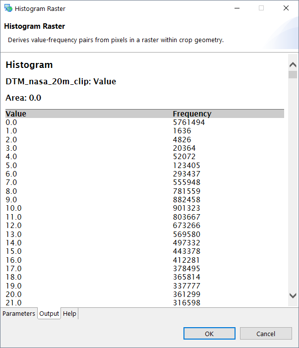
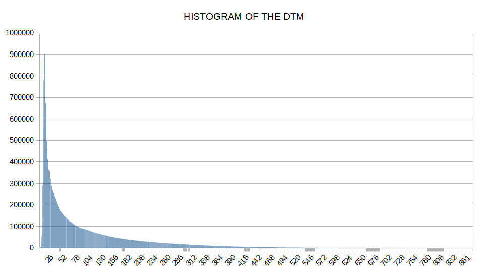
Histogram Raster is a tool which calculates the information to be used to create a histogram of the content of the raster layer. In particular, this tool calculates and prints the number of cells of each different value in the map. These values can be used to display a histogram chart, just select and copy and paste them in a spreadsheet. It is available in the section:

Raster Tools → Descriptive Statistics

double click on the Histogram raster entry. The required input parameters are:

1. Input Raster layer: select the raster layer to elaborate from the list of the raster layers available in the Map

2. Band Index (optional): optional value of band index to use for multiple band layers, otherwise leave it at 0

3. Crop Geometry (optional): a reference for "clipping" a custom area of the raster layer if you need to extract the information on a subset of the complete raster; click the at the end of the line to choose how to select it:

   • Point

   • LineString: selects the boundary from the area_of_interest Layer’s Extent

   • Polygon: selects the polygon from the area_of_interest Layer’s Extent

   • Geometry from Layers…​: selects the layer and feature ID of the polygon to use for delimiting the new vector layer.

Figure 19. Execution of the Histogram Raster.

Figure 20. Output of the Histogram Raster.

Figure 21. Graphic output of the Histogram Raster.

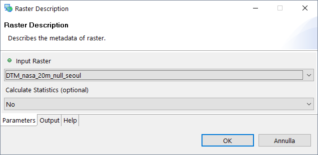
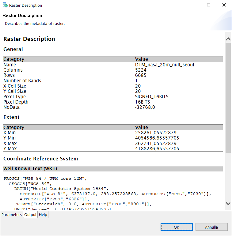
Raster Description is a tool which can be used to have a first description of the general metadata of the selected raster. The metadata visualized are: Name, Columns, Rows, Number of Bands, X-Y Cell Size, Pixel Type, Pixel Depth, NoData Value, the whole Extent and the CRS (Coordinate Reference System). This tool gives also the possibility to directly perform Summary Statistics.

Figure 22. Execution of the Raster Description.

Figure 23. Output of the Raster Description.

3.1. The Normalized Difference Vegetation Index

From an ecological and environmental point of view an interesting index which can be calculated from Landsat8 images is the NDVI. The Normalized Difference Vegetation Index is a simple graphical indicator that can be used to analyse remote sensing measurements and assess whether there is live green vegetation on the surface of the analysed area. The expression of the NDVI is:

\(NDVI={\frac {(NIR-Red)}{(NIR+Red)}}\)

The Processing Toolbox contains a module to directly perform this index, it is available in the section:

Raster Tools → Math → NDVI

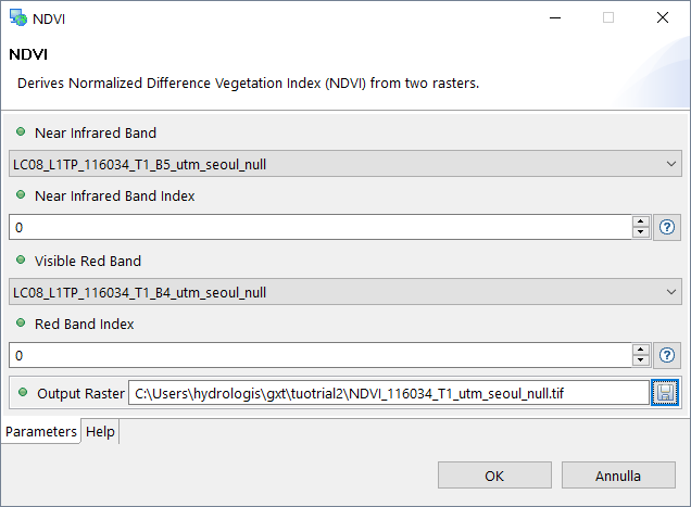
The required input parameters are:

1. Near Infrared Band layer: select the raster layer containing the NIR information from the list of the raster layers available in the Map
2. Near Infrared Band Index: optional value of band index to use for multiple band layers, otherwise leave it at 0
3. Visible Red Band layer: select the raster layer containing the VIS red information from the list of the raster layers available in the Map
4. Red Band Index: optional value of band index to use for multiple band layers, otherwise leave it at 0
5. Output Raster: the path and name of the output raster layer.

The output raster layer will be shown with an homogenious

Figure 24. Execution of the NDVI.

To understand the content of the NDVI map it is recommended to do some statistical analysis on it, please run the modules for Descriptive Statistics on this map as described in the previous paragraph:

1. Summary Statistics for Raster
2. Histogram

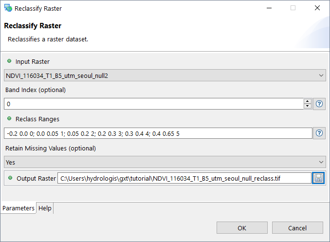
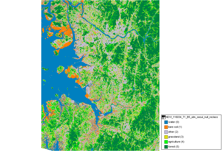
Reclassify Raster is used to reassign a value, a range of values, or a list of values in a raster to new output values. Reclassification is useful to assign each value (pixel) of a raster map to a category in a list of predefined categories. In our example NDVI values are in the range from -0.2 to 0.64, but these values are a bit complicated to understand for a wide public, so a reclassification process will be useful. From bibliography studies and without a real validation we can use, for example, the following ranges for reclassification:

Table 1. Values and classes used for reclassifying NDVI raster layer

CLASS	MAX VALUE	MIN VALUE	DESC
0	-0.5	0.0	water
1	0.0	0.05	bare soil
2	0.05	0.2	other (roof, city, …​)
3	0.2	0.3	grassland
4	0.3	0.4	agriculture
5	0.4	0.7	forest

Reclassification is available in the section:

Raster Tools → Reclass

double click on the Reclassify Raster entry. The required input parameters are:

1. Input Raster layer: select the raster layer to reclassify from the list of the raster layers available in the Map

2. Band Index (optional): optional value of band index to use for multiple band layers, otherwise leave it at 0

3. Reclass Ranges: the ranges of the different categories in which to assign each value of the raster map; write here the list of categories and intervals or click the at the end of the line to choose how to select it:

   • Build expression: opens the Expression Builder Dialog where it is possible to insert a formula to assign the values to a class

   • Select Multiple Fields: opens the Multiple Fields Selector where it is possible to select a vector layer and assign the values of the raster layer to a set or to all the different values of one of its fields

   • Select Statistical Fields: opens the Statistics Fields Selector where it is possible to select a vector layer and assign the values of the raster layer to a statistic extraction of the values of one of its fields

4. Retain Missing Values: defines whether missing values in the reclass table maintain their value (true) or get mapped to NoData (false)

5. Output Raster: the path and name of the output raster layer.

To use the categories of the table above we can write them directly in the text field of the Reclass Ranges in the form of:

-0.2 0.0 0; 0.0 0.05 1; 0.05 0.2 2; 0.2 0.3 3; 0.3 0.4 4; 0.4 0.65 5

Figure 25. Execution of the Reclassify Raster.

After reclassification the visualization of the NDVI map will be more clear and it is also easier to style it using a Unique Values color table.

Other bands of the Landsat8 images are interesting for an ecological point of view, before going on with the next operations please proceed to reclassify also the map of band 5 representing the NIR (Near Infra Red) which is important for ecology studies because healthy plants reflect this frequency. Usually the bright features of this band are parks and other heavily irrigated vegetation.

Figure 26. NDVI map styled after reclassification.

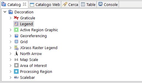
Template:Note Legend of the visualized layers in uDig is available in the Decoration folder of the catalog. To add the legend to the map go in the Catalog View and scroll until Decoration item is visualized, then click on the arrow before the name to show its content. Double click on Legend to add it directly to the Map View. To define a personalized style for the legend select the Legend layer form the Layers View and access the style editor questionmark

Figure 27. Access to the Legend item from the Catalog View.

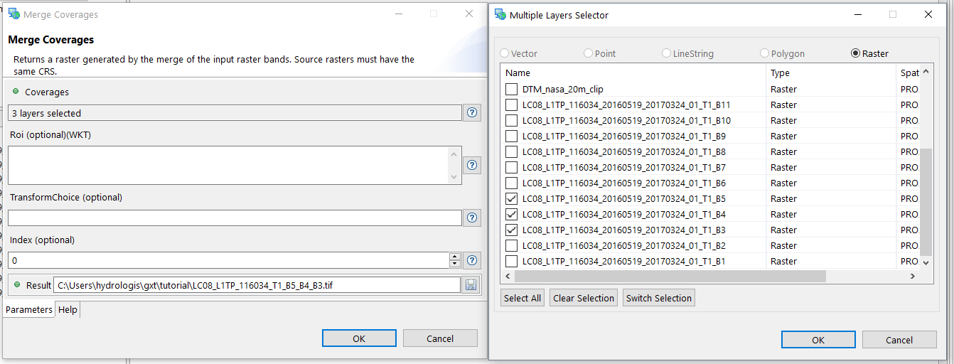
Band Merge is an other interesting tool for analysing satellite data expecially Landsat8 images which are divided into 11 different images. Possible combination of these images can give the user interesting information about the elements on the surface. For example the combination of bands of Red, Green and Blue (RGB) is used to obtain a true color map, useful also for studying aquatic habitats. To do this we can use the Band Merge tool available in:

GeoTools Processes → Raster processes

double click on the Band Merge entry. The required input parameters are:

1. Coverages: select the input raster layers of the different bands to merge from the list of the raster layers available in the Map, click the at the end of the line to select them from the Multiple Layers Selector

2. ROI (optional)(WKT): optional value of the region of interest if you want to run the process on a smallest area rather than all images click the at the end of the line to choose how to select it:

   • Point

   • LineString: selects the boundary from the area_of_interest Layer’s Extent

   • Polygon: selects the polygon from the area_of_interest Layer’s Extent

   • Geometry from Layers…​: selects the layer and feature ID of the polygon to use for delimiting the new vector layer

3. TransformChoice (optional): choose the transformation to use in case of a transformation of the original input data is needed; insert the expression of the transformation here or click the at the end of the line to choose how to define it:

   • Build Expression: opens the Expression Builder Dialog to write the transformation using the available tools

   • Select Multiple Fields: opens the Multiple Fields Selector where it is possible to select the fields of a vector layer as parameters of the transformation

   • Select Statistical Fields: opens the Statistics Fields Selector where it is possible to selectthe fields of a vector layer as parameters of the transformation

4. Index (optional): the index used by the TransforChoice parameter needed only if there is a TransforChoice

5. Result: the path and name of the output merged raster layer.

Figure 28. Execution of the Band Merge with the detail of the window were to select the input raster layers of the different bands, The example of the true color map.

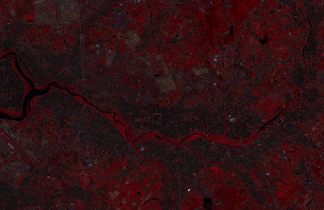
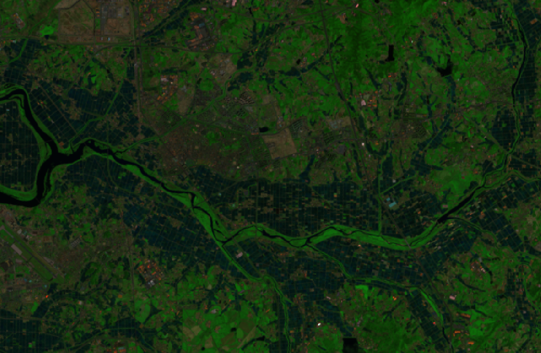
Other interesting maps che be evaluated using the merging tools combining the bands:

• bands 5,4,3 to have clearer boundaries of the water bodies and stess the difference of the vegetation types
• bands 5,6,4 which is crisper than the previous one where different vegetation types can be more clearly defined and land/water interface more clear
• bands 7,5,3 similar to the previous one but in this case the vegetation appears green
• bands 6.5.2 specific to visualize agricultural vegetation.

Please proceed in the elaboration of these other maps and try to define different styles of visualization and to identify the differences and the peculiarities of each single map. The following images show some results.

Figure 29. Visualization of the output true color map of merging bands 2,3,4.

Figure 30. Visualization of the output true color map of merging bands 3,4,5.

Figure 31. Visualization of the output true color map of merging bands 3,5,7.

Analysis of the Digital Terrain Model

The raster of the Digital Terrain Model (DTM) contains the values of the elevation of the terrain at the given resolution. This information can be used to perform geomorphological analysis on the terrain (slope, curvature, …​) or to link the information of the elevation to other discrete data.

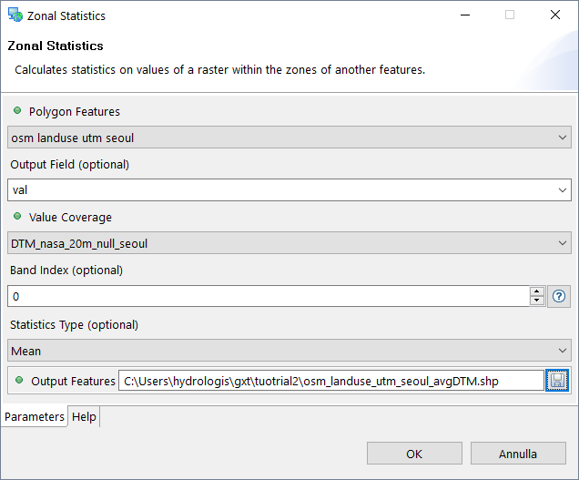
For example, it could be useful to analyse the connection between a discrete information (the land use) and the elevation or the slope of the terrain. The tool to perform this operation is the Zonal Statistics which is available in:

Raster Tools → Zonal Tools → Zonal Statistics

The required input parameters are:

1. Polygon Features layer: select the vector layer of the landuse crop on the area of interest from the list of the vector layers available in the Map

2. Output Field (optional): name of the new field that will be added to the input polygon layer containing the results

3. Value Coverage layer: select the raster layer containing the values for which to perform zonal statistics on the polygons, in this case the DTM

4. Band Index (optional): optional value of band index to use for multiple band layers, otherwise leave it at 0

5. Statistics Type (optional): the statistical analysis on the raster values for each polygon of the features layer, you can choose between:

   • Count

   • Sum

   • Mean

   • Minimum

   • Maximum

   • Range

   • Standard Deviation

6. Output Features layer: the path and name of the output polygon layer containing the additional field with the statistics.

'	Before proceeding with the Zonal Statistics it is recommended to set zero values of the DTM map (0.0) to null with the Set Null tool as described in the previous chapter.

The example is performed considering the average value of elevation in each polygon as specified in the following figures.

Figure 32. Execution of the Zonal Statistics.

The output will be a vector layer with the same features of the input one with two additional attributes (visible in the Table view) named Val and Cell_Area.

Figure 33. Output of the Zonal Statistics of the DTM on the LandUse polygons with a tematic styling considering the average elevation of the polygons.

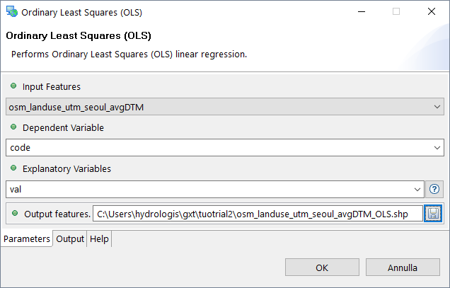
To analyse the results of the zonal statistics it is possible to use a spatial correlation which can be evaluated using the Ordinary Linear Regression (OLS) considering the two variables, landuse (code) and average elevation (val) respectively as dependent and independent variables. This tool is available in:

Spatial Statistics → Spatial Relationships → Ordinary Least Squares

The required input parameters are:

1. Input Features layer: select the vector layer of the landuse crop on the area of interest from the list of the vector layers available in the Map
2. Dependent Variable: select the field of the input polygon layer containing the information about the dependent variable (i.e. code)
3. Explanatory Variable: select the field of the input polygon layer containing the information about the explanatory variable (i.e. value)
4. Output Features layer: the path and name of the output polygon layer containing the additional field of the OLS.

Figure 34. Execution of the Ordinary Least Squares.

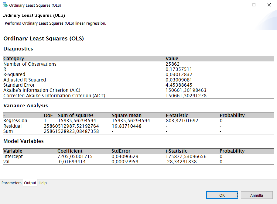
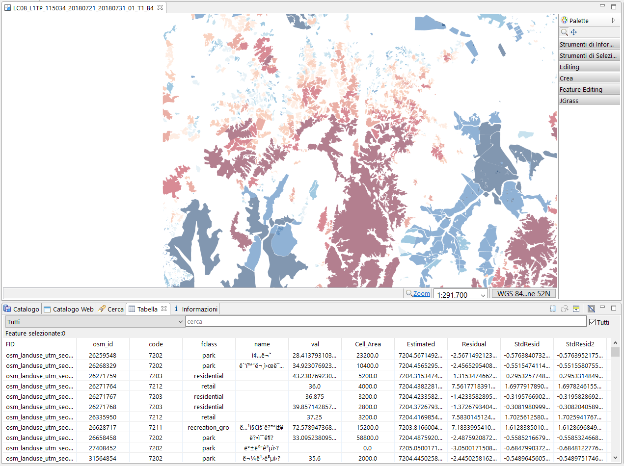
The output will be a vector layer with the same features of the input one with two additional attributes (visible in the Table view) named Estimated, Residual, StdResid and *StdResid2. As you can see from the following image the *R^2 is very low so basically there is no linear correlation between the two variables.

Figure 35. Output of the Ordinary Least Squares of the elevation on the landuse.

Figure 36. Output of the Ordinary Least Squares of the elevation on the landuse.

It is possible to do this kind of evaluations also considering a different independent variable for example the slope of the terrain.

4.1. Morphological analysis on DTM

The Processing Toolbox contains some tools for basic morphological analysis on a Digital Terrain Model (DTM). Example of these tools are the slope and the curvature models which will be analysed in the following sections.

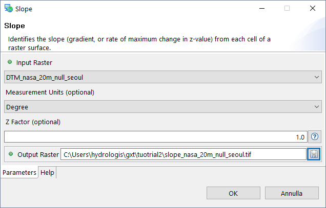
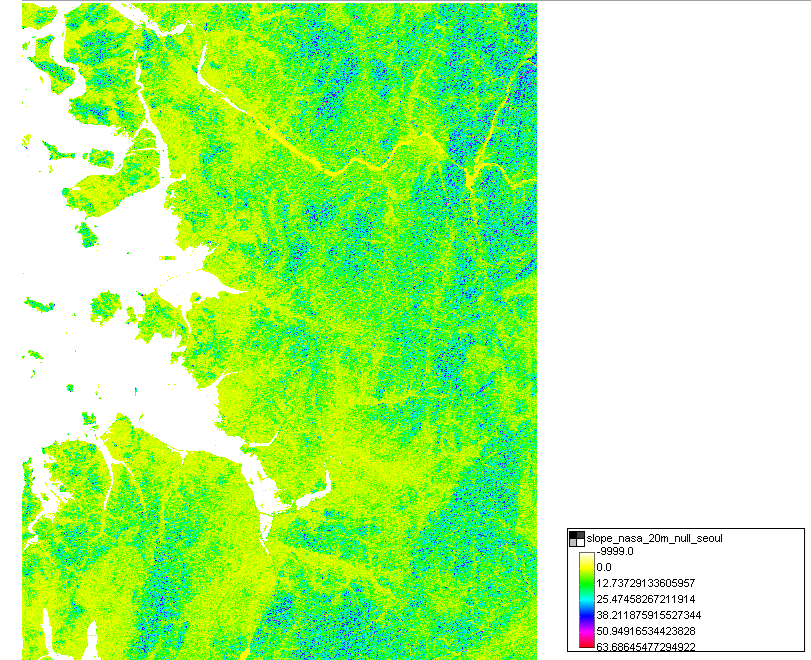
Slope tool identifies the slope of the terrain as the gradient, or in other words, the rate of maximum change in z-value from each cell of a raster surface following the drainage directions. The module is available in:

Raster Tools → Surface Analysis → Slope

The required input parameters are:

1. Input Raster layer: select the raster layer of the DTM for which to evaluate the maximum gradients of the surface from the list of the vector layers available in the Map
2. Measurement Units (optional): select the unit of measurement for the output slope raster map between the given options (Degree, Percentrise)
3. Z factor (optional): specify the number of ground x,y units in one surface Z unit; this value can be constant or given as field in a vector layer (you can select the vector layer and the other parameters using the at the end of the line
4. Output Raster layer: the path and name of the output raster layer containing the slope.

Figure 37. Execution of the Slope.

Figure 38. Output of the Slope in degree.

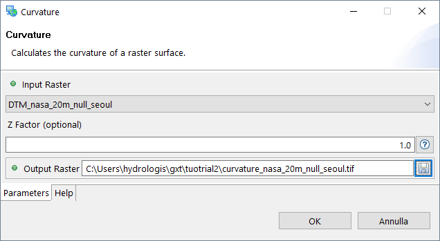
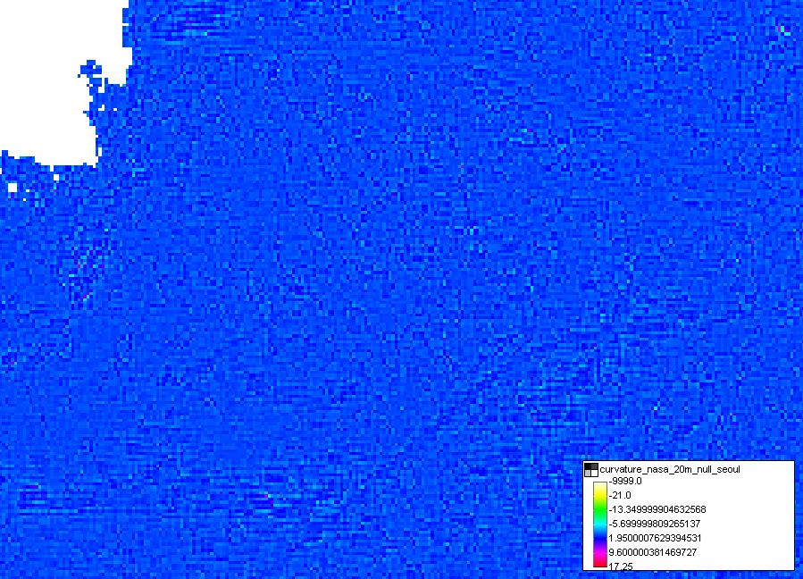
Curvature tool calculates the curvature of a raster surface (DTM). The module is available in:

Raster Tools → Surface Analysis → Curvature

The required input parameters are:

1. Input Raster layer: select the raster layer of the DTM for which to evaluate the curvature of the surface from the list of the vector layers available in the Map
2. Z Factor (optional): specify the number of ground x,y units in one surface Z unit; this value can be constant or given as field in a vector layer (you can select the vector layer and the other parameters using the at the end of the line)
3. Output Raster layer: the path and name of the output raster layer containing the curvature.

Figure 39. Execution of the Curvature.

Figure 40. Output of the Curvature of the terrain.

The Processing Toolbox contains two modules to quantify the topographic heterogeneity of a surface, one general and one more specific for terrain.

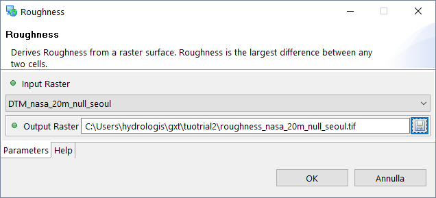
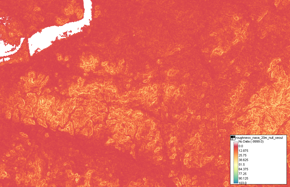
Roughness, represents the general tool calculate the roughness of the surface as the maximum difference between the values in two cells. The module is available in:

Raster Tools → Surface Analysis → Roughness

The required input parameters are:

1. Input Raster layer: select the raster layer of the DTM for which to evaluate the roughness of the surface from the list of the raster layers available in the Map
2. Output Raster layer: the path and name of the output raster layer containing the roughness of the surface.

Figure 41. Execution of the Roughness.

Figure 42. Output of the Roughness of the terrain as a general surface.

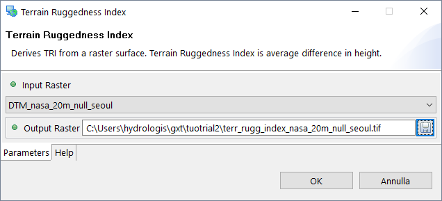
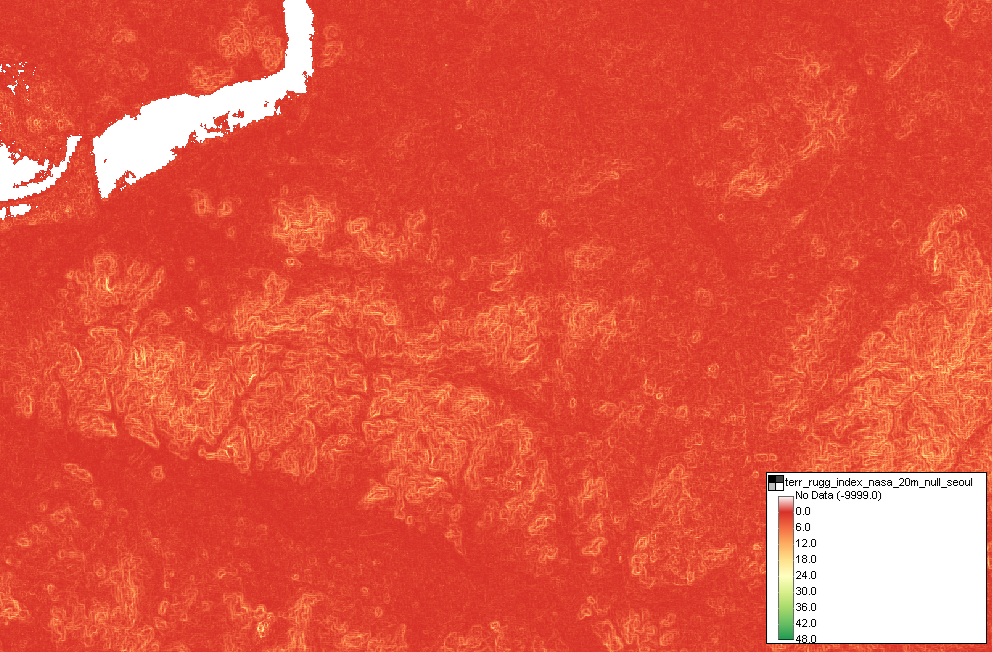
Roughness, represents the tool specific to evaluate the ruggedness of the terrain (DTM) as the average difference in height. The module is available in:

Raster Tools → Surface Analysis → Terrain Ruggedness Index

The required input parameters are:

1. Input Raster layer: select the raster layer of the DTM for which to evaluate the ruggedness from the list of the raster layers available in the Map
2. Output Raster layer: the path and name of the output raster layer containing the Terrain Ruggedness Index.

Figure 43. Execution of the Terrain Ruggedness Index.

Figure 44. Output of the Terrain Ruggedness Index of the terrain.

'	As shown in the previous images, considering the DTM the two variables (roughness and Terrain Ruggedness Index) have different values but the same behaviour.

It is now possible to evaluate the correlation between the Land Use and all these variables, calculated as raster maps (slope, curvature, roughness and Terrain Ruggedness Index) as previously done with the DTM using the Zonal Statistics and Ordinary Least Squares (OLS) tools.

4.2. Add information to vector layers

There is another possibility to extract continuous information over a surface from raster layers to discrete points in a vector layer.

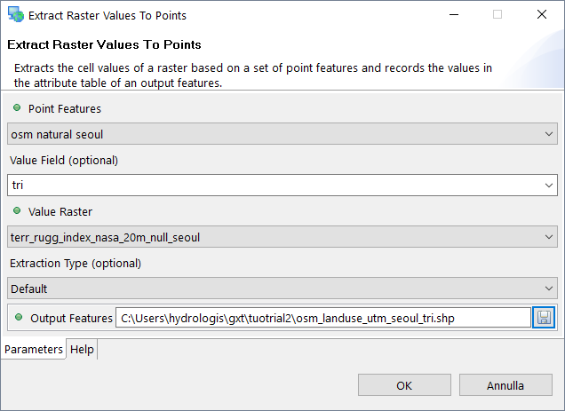
Extract Raster Values to Points extracts the cell values of a raster for a set of points and stores these values in the attribute table of an output vector layer. The module is available in:

General Tools → Calculation → Extract Raster Values to Points

The required input parameters are:

1. Point Features layer: select the vector layer of the natural sites for which to extract the values from the list of the vector layers available in the Map
2. Value Field (optional): name of the field containing the values of the raster layer in the new vector layer
3. Value Raster layer: select the raster layer (i.e. the Terrain Ruggedness Index, Slope) of from which to extract the values to add to the vector layer from the list of the raster layers available in the Map
4. Extraction Type (optional): select the value to extract from the raster layer; the options are: Default, SlopeAsDegree, SlopeAsPercentrise, Aspect
5. Output Features layer: the path and name of the output vector layer containing the additional field with raster values.

Figure 45. Execution of the Extract Raster Values to Points.

Figure 46. Output of the Extract Raster Values to Points.

Working with vector data

Geospatial vector layers are a representation of the world using points, lines, and polygons. Vector models usually are used for storing data that has discrete boundaries stored in an attribute table. The attribute table is definitely a table containing for each feature the values of the list of attributes available, some of them can also be null or zero.

Analysis on vector data can be performed on geometries or on some attribute and, in general, are not so memory expensive like the rasters analysis. In this chapter we will see some of the possibilities available in the Processing Toolbox.

5.1. Analysis of single layers

The Nearest Neighbor Index (NNI) is based on the average distance from each feature to its nearest neighboring feature. It measures the spatial distribution of a pattern to evaluate if it is regularly dispersed (=probably planned), randomly dispersed, or clustered. It is normally used for spatial geography (study of landscapes, human settlements, etc).

The NNI is expressed as the ratio of the observed distance divided by the expected distance. The expected distance is the average distance between neighbors in a hypothetical random distribution:

• NNI < 1 : the pattern exhibits clustering
• NNI = 1 : randomly dispersed pattern
• NNI > 1 : the trend of the distribution is toward dispersion or competition
• NNI = 2.15 : regularly dispersed /uniform pattern.

The module is available in:

Spatial Statistics → Point Pattern Analysis → Nearest Neighbor Index

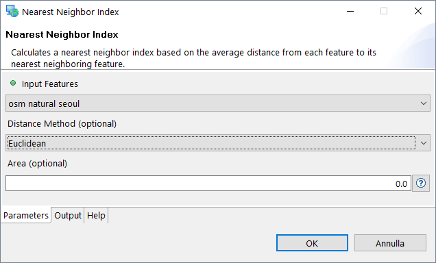
The required input parameters are:

1. Input Features layer: select the vector layer of the Natural Points for which to evaluate the NNI from the list of the vector layers available in the Map
2. Distance Method (optional): method to evaluate the distance between the single features and each neighboring feature, the available options are Euclidean and Manhattan
3. Area (optional): the area of the study region (you can select the vector layer to use to evaluate the area using the at the end of the line).

Figure 47. Execution of the Nearest Neighbor Index.

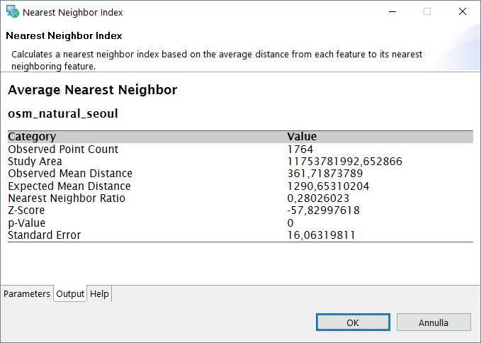
The Z score value is a measure of statistical significance to evaluate whether or not to reject the null hypothesis (in this case, randomly distributed points). If an area value is not specified, then the area of the minimum enclosing rectangle around all the features is used. The result is a report containing the NNI of the elements in the input layer over the specified area. The variables reported are:

• Observed Point Count
• Study Area
• Observed Mean Distance
• Expected Mean Distance
• Nearest Neighbor Index
• Z-Score
• p-Value
• Standard Error

Figure 48. Output of the Nearest Neighbor Index of the Natural Points.

In this case the Z-Score shows that there is not statistical significance in this evaluation, even if the NNI 0.3 means that the distribution exhibits some clusters.

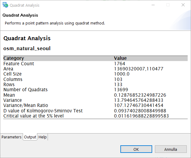
Other methods to perform point pattern analysis is the quadrant method using the Quadrant Analysis tool. This technique consists in dividing the study area into sub-regions (aka quadrats). Then, the point density is computed for each quadrat by dividing the number of points in each quadrant by the quadrant’s area. The version integrated in the Processing Toolbox consider only squares quadrants. The module is available in:

Spatial Statistics → Point Pattern Analysis → Quadrant Analysis

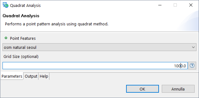
The required input parameters are:

1. Point Features layer: select the vector layer of the Natural Points for which to perform the quadrant analysis from the list of the vector layers available in the Map
2. Grid Size (optional): the dimension of the quadrants in which to divide the area of the study region (you can select the vector layer to use to define this value using the at the end of the line).

'

The quadrant size influence the measure of local density and must be chosen with care. If the quadrants size is too small there is the risk of having many quadrants with no points which may prove uninformative. In case of too large quadrants size there is the risk of missing particular changes in spatial density distributions. An other peculiarity of this method is that the quadrant regions do not have to take on a uniform pattern across the study area.

Figure 49. Execution of the Quadrant Analysis.

Figure 50. Output of the Quadrant Analysis of the Natural Points.

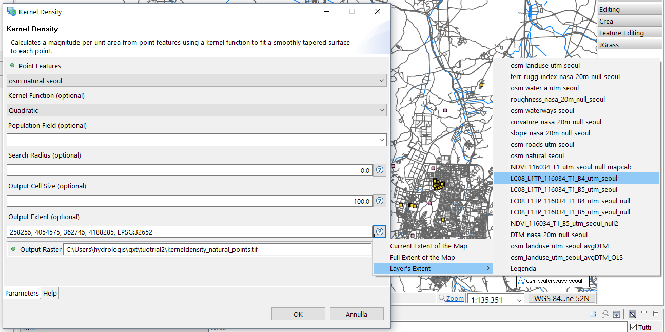
Kernel Density extend the quadrant methodology, like the quadrant density, it computes a localized density for subsets of the study area, but unlike the quadrant density, the sub-regions overlap one another providing a moving sub-region window. This moving window is defined by a kernel. In this way, the kernel density approach generates a grid of density values based on cell size smaller than the kernel window. Each cell is assigned the density value computed for the kernel window centered on that cell. The output is a raster containing the density values.

The kernel defines the shape and size of the window, but it can also weight the points following a defined kernel function. The most popular kernel functions assign weights to points that are inversely proportional to their distances to the kernel window center. The simplest of functions is a basic kernel where each point in the kernel window is assigned equal weight.

The module is available in:

Raster Tools → Density → Kernel Density

The required input parameters are:

1. Point Features layer: select the vector layer of the Natural Points for which to perform the kernel density from the list of the vector layers available in the Map

2. Kernel Function (optional): the function to use to weight the points in the kernel

3. Population Field (optional): the field containing the population value for each feature, if available

4. Search Value (optional): the radius of the kernel used to calculate the density (you can select the vector layer to use to define this value using the at the end of the line)

5. Output Cell Size (optional): the value of the cell size of the output raster (you can select the vector layer to use to define this value using the at the end of the line)

6. Output Extent (optional): the region of the output raster (specify the boundaries), you can select the options available to define this value using the at the end of the line:

   • Current Extent of the Map

   • Full Extent of the Map

   • Layers Extent: select the raster or vector layer from the list of all the layers available in the Map

   • Output Raster layer: the path and name of the output raster layer containing the roughness of the surface.

Figure 51. Execution of the Kernel Density.

Figure 52. Output of the Kernel Density of the Natural Points.

'	This elaboration uses much memory and it requires lot of time to finish. Please be careful of delimiting the extent of the elaboration and a reasonable value for the output cell size.

5.2. Combination of multiple layers

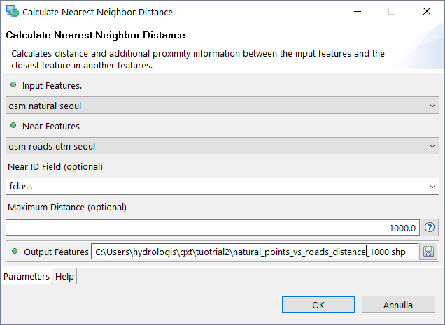
In environmental studies it is often useful to perform analysis on multiple layers to understand if there is a correlation between different discrete information. An example of this is the evaluation of the distance between the features in a layer with the nearing neighboring features in a second layer. Calculate Nearest Neighbor Distance calculates the distance between each feature in the input layer and the closer feature in a second layer. The module is available in:

General Tools → Proximity Analysis → Calculate Nearest Neighbor Distance

The required input parameters are:

1. Input Features layer: select the vector layer of the Natural Points for which to calculate the distance from the list of the vector layers available in the Map
2. Near Features layer: select the vector layer of the Roads or Water Lines to use as reference to calculate the distance from the features of the Input Layer, from the list of the vector layers available in the Map
3. Near ID Field (optional): the field containing the ID of the nearest feature (output layer)
4. Maximum distance (optional): the value of the maximum distance to explore for searching the feature (you can select the vector layer to use to define this value using the at the end of the line)
5. Output Features layer: the path and name of the output vector layer containing the proximity information for each feature of the Input Features layer.

Figure 53. Execution of the Calculate Nearest Neighbor Distance vs the Roads.

Figure 54. Output of the Calculate Nearest Neighbor Distance of the Natural Points vs the Roads.

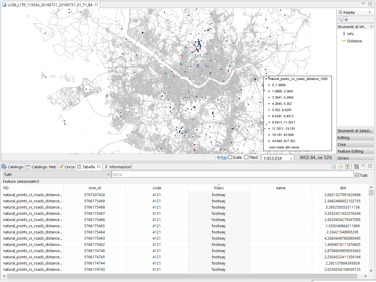
'	The output of the Nearest Neighbor Distance tool shows clearly that the closest road to the natural points are footways.

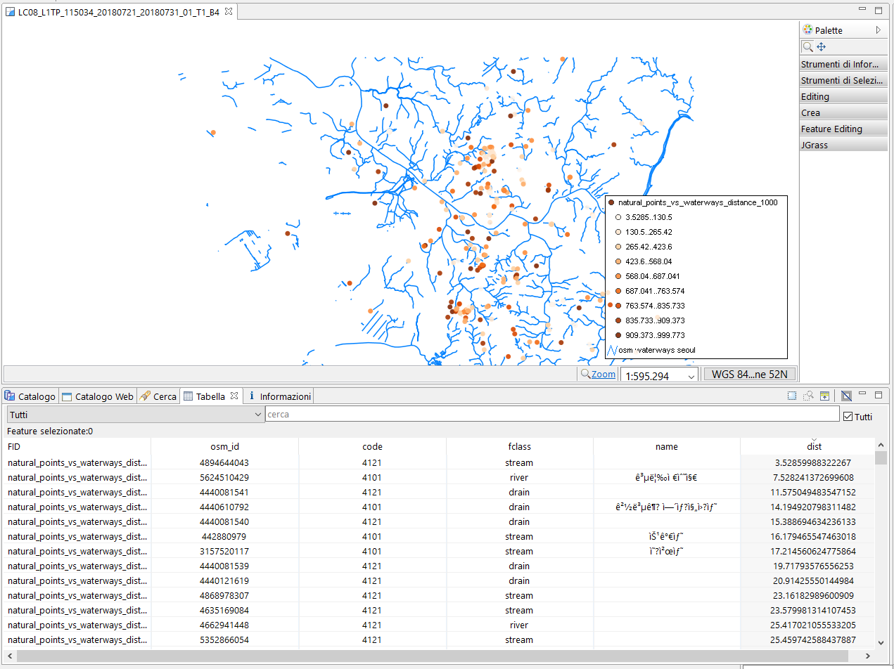
Now it is possible to use the same tool to perform the distance between the Natural Points and the Water Lines. The result is the following:

Figure 55. Output of the Calculate Nearest Neighbor Distance of the Water Lines vs the Roads.

5.3. Summary of statistics on vector layers

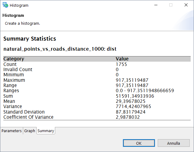
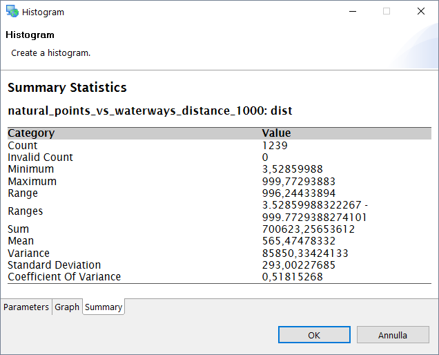
The Processing Toolbox contains a set of tools which can be used to create a statistics report on the results obtained for the different analysis. In this example we can use some tools to realize charts on the distance calculated between the Natural Points and the Roads or the Water Lines.

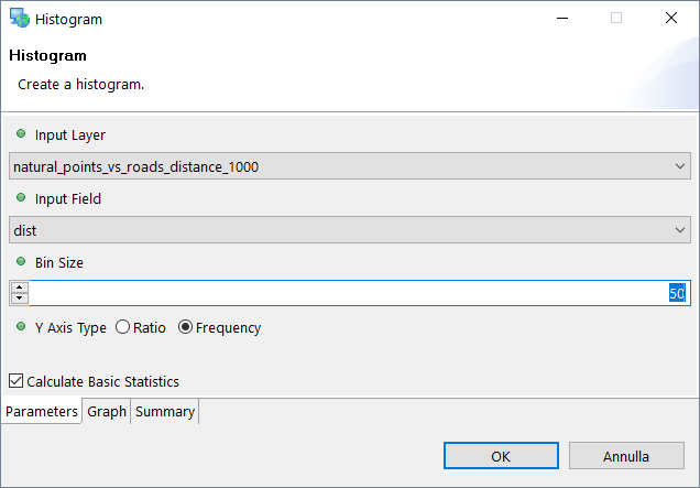
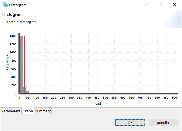
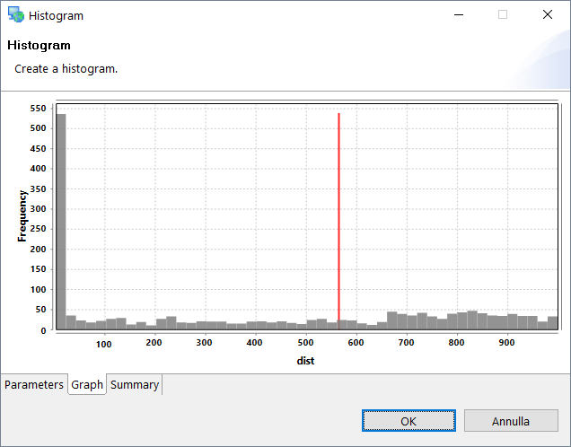
Histogram is a tool to create a histogram chart on a defined field of the selected vector layer. The module is available in:

General Tools → Graph → Histogram

The required input parameters are:

1. Input Layer: select the vector layer of the Natural Points with road distance for which to create the histogram from the list of the vector layers available in the Map
2. Input Field: select the field of the vector layer to use as reference for the chart from the list of the layers attributes (only numeric attributes are considered)
3. Bin Size: the number of bins in which to divide the range of the values in the input field
4. Y Axis Type: select if you want the values of the Ratio or the Frequency of the values in the Y axis.

Figure 56. Execution of the Histogram on the distance between the Natural Points and the Roads.

Figure 57. Output of the Histogram on the distance between the Natural Points and the Roads.

Figure 58. Output of the Histogram on the distance between the Natural Points and the Roads.

Now it is possible to use the same tool to perform the distance between the Natural Points and the Water Lines.

Figure 59. Output of the Histogram on the distance between the Natural Points and the Water Lines.

Figure 60. Output of the Histogram on the distance between the Natural Points and the Water Lines.

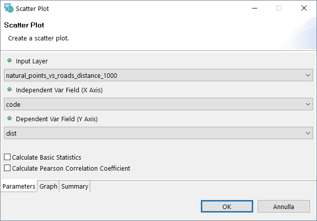
Scattered Plot is a tool to create a scattered plot chart on a defined field of the selected vector layer using an other field as reference variable. The module is available in:

General Tools → Graph → Scattered Plot

The required input parameters are:

1. Input Layer: select the vector layer of the Natural Points with road distance for which to create the scattered plot from the list of the vector layers available in the Map
2. Independent Var Field (X Axis): select the field of the input vector layer to use as independent variable on the X axis (only numeric fields can be accepted)
3. Dependent Var Field (X Axis): select the field of the input vector layer to use as dependent variable on the Y axis (only numeric fields can be accepted)
4. Calculate Basic Statistics: select this chechbox to extract also the basic statistics information in the same process
5. Calculate Pearson Correlation Coefficient: select this chechbox to extract also the information related to the Pearson Correlation Coefficient in the same process.

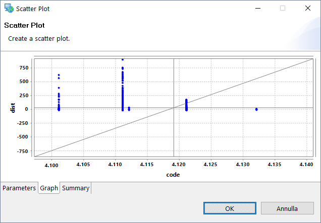
Figure 61. Execution of the Scattered Plot on the distance between the Natural Points and the _Roads.

Figure 62. Output of the Scattered Plot on the distance between the Natural Points and the _Roads.

'	the Independent Variable, X in this case is the code representing the category of the road.

Version 0.1